Bayes Factor comparison

Last updated: 2024-11-20

Checks: 6 1

Knit directory: survival-susie/

This reproducible R Markdown analysis was created with workflowr (version 1.7.0). The Checks tab describes the reproducibility checks that were applied when the results were created. The Past versions tab lists the development history.

R Markdown file: up-to-date

Great! Since the R Markdown file has been committed to the Git repository, you know the exact version of the code that produced these results.

Environment: empty

Great job! The global environment was empty. Objects defined in the global environment can affect the analysis in your R Markdown file in unknown ways. For reproduciblity it’s best to always run the code in an empty environment.

Seed: set.seed(20230201)

The command set.seed(20230201) was run prior to running the code in the R Markdown file. Setting a seed ensures that any results that rely on randomness, e.g. subsampling or permutations, are reproducible.

Session information: recorded

Great job! Recording the operating system, R version, and package versions is critical for reproducibility.

Cache: none

Nice! There were no cached chunks for this analysis, so you can be confident that you successfully produced the results during this run.

File paths: absolute

Using absolute paths to the files within your workflowr project makes it difficult for you and others to run your code on a different machine. Change the absolute path(s) below to the suggested relative path(s) to make your code more reproducible.

absolute	relative
/project2/mstephens/yunqiyang/surv-susie/survival-susie/output/bf_comparison_b_1_n_500000.pdf	output/bf_comparison_b_1_n_500000.pdf
/project2/mstephens/yunqiyang/surv-susie/survival-susie/output/bf_comparison_b_0.1_n_500000.pdf	output/bf_comparison_b_0.1_n_500000.pdf
/project2/mstephens/yunqiyang/surv-susie/survival-susie/output/bf_comparison_b_0.01_n_500000.pdf	output/bf_comparison_b_0.01_n_500000.pdf

Repository version: 6f59843

Great! You are using Git for version control. Tracking code development and connecting the code version to the results is critical for reproducibility.

The results in this page were generated with repository version 6f59843. See the Past versions tab to see a history of the changes made to the R Markdown and HTML files.

Note that you need to be careful to ensure that all relevant files for the analysis have been committed to Git prior to generating the results (you can use wflow_publish or wflow_git_commit). workflowr only checks the R Markdown file, but you know if there are other scripts or data files that it depends on. Below is the status of the Git repository when the results were generated:


Ignored files:
    Ignored:    .RData
    Ignored:    .Rhistory
    Ignored:    .Rproj.user/

Untracked files:
    Untracked:  analysis/time_gh.Rmd
    Untracked:  output/bf_comparison_b_1_n_500000.pdf

Unstaged changes:
    Modified:   analysis/bf_comparison.Rmd
    Deleted:    analysis/calibration_large_sample.Rmd
    Modified:   analysis/check_bf.Rmd
    Modified:   analysis/coxph_na.Rmd
    Modified:   analysis/pip_default_iter_gtex.Rmd
    Modified:   code/pip.R
    Modified:   output/bf_comparison.pdf
    Modified:   output/bf_comparison_b_0.01_n_500000.pdf
    Modified:   output/bf_comparison_b_0.1_n_500000.pdf
    Modified:   output/bf_defense.pdf
    Modified:   output/bf_different_bhat_large_n.pdf
    Modified:   output/bf_different_bhat_small_n.pdf
    Modified:   output/bf_different_n_large_b.pdf
    Deleted:    output/pip_combined.Rmd
    Modified:   output/pip_gtex.pdf
    Modified:   output/pip_ukb.pdf

Note that any generated files, e.g. HTML, png, CSS, etc., are not included in this status report because it is ok for generated content to have uncommitted changes.

These are the previous versions of the repository in which changes were made to the R Markdown (analysis/bf_comparison2.Rmd) and HTML (docs/bf_comparison2.html) files. If you’ve configured a remote Git repository (see ?wflow_git_remote), click on the hyperlinks in the table below to view the files as they were in that past version.

File	Version	Author	Date	Message
Rmd	6f59843	yunqi yang	2024-11-20	wflow_publish("analysis/bf_comparison2.Rmd")
html	410628d	yunqi yang	2024-10-11	Build site.
Rmd	04c2e21	yunqi yang	2024-10-11	wflow_publish("analysis/bf_comparison2.Rmd")
html	c219afc	yunqi yang	2024-10-11	Build site.
Rmd	19a7ce3	yunqi yang	2024-10-11	wflow_publish("analysis/bf_comparison2.Rmd")
html	8a1ddda	yunqi yang	2024-10-07	Build site.
Rmd	08f38c4	yunqi yang	2024-10-07	wflow_publish("analysis/bf_comparison2.Rmd")
html	6445624	yunqi yang	2024-09-18	Build site.
Rmd	a68068a	yunqi yang	2024-09-18	wflow_publish("analysis/bf_comparison2.Rmd")
html	5b1f3bf	yunqi yang	2024-09-15	Build site.
Rmd	cf8b1c2	yunqi yang	2024-09-15	wflow_publish("analysis/bf_comparison2.Rmd")
Rmd	9d07e13	yunqi yang	2024-09-04	update bf result
html	546c2bf	yunqi yang	2024-08-26	Build site.
Rmd	f39a9fa	yunqi yang	2024-08-26	wflow_publish("analysis/bf_comparison2.Rmd")
html	8e45b7b	yunqi yang	2024-08-25	Build site.
Rmd	540034b	yunqi yang	2024-08-25	wflow_publish("analysis/bf_comparison2.Rmd")
html	a066bd5	yunqi yang	2024-08-22	Build site.
Rmd	ff1c9e9	yunqi yang	2024-08-22	wflow_publish("analysis/bf_comparison2.Rmd")
html	0a749f7	yunqi yang	2024-08-20	Build site.
Rmd	f2b94f6	yunqi yang	2024-08-20	wflow_publish("analysis/bf_comparison2.Rmd")
html	0c00f19	yunqi yang	2024-07-30	Build site.
Rmd	d57da75	yunqi yang	2024-07-30	wflow_publish("analysis/bf_comparison2.Rmd")
html	46926b2	yunqi yang	2024-07-30	Build site.
Rmd	5845f48	yunqi yang	2024-07-30	wflow_publish("analysis/bf_comparison2.Rmd")
html	3ec6bec	yunqi yang	2024-07-30	Build site.
Rmd	1dc809b	yunqi yang	2024-07-30	wflow_publish("analysis/bf_comparison2.Rmd")
html	09175d7	yunqi yang	2024-07-30	Build site.
Rmd	f02670e	yunqi yang	2024-07-30	wflow_publish("analysis/bf_comparison2.Rmd")
html	d88a721	yunqi yang	2024-07-30	Build site.
Rmd	3d8ee7d	yunqi yang	2024-07-30	wflow_publish("analysis/bf_comparison2.Rmd")
html	e967833	yunqi yang	2024-07-30	Build site.
Rmd	4f6011c	yunqi yang	2024-07-30	wflow_publish("analysis/bf_comparison2.Rmd")
html	446abfc	yunqi yang	2024-07-30	Build site.
Rmd	648758a	yunqi yang	2024-07-30	wflow_publish("analysis/bf_comparison2.Rmd")
html	9a0ac2e	yunqi yang	2024-07-25	Build site.
Rmd	c49d023	yunqi yang	2024-07-25	wflow_publish("analysis/bf_comparison2.Rmd")
html	a052a70	yunqi yang	2024-07-25	Build site.
Rmd	9e875e9	yunqi yang	2024-07-25	wflow_publish("analysis/bf_comparison2.Rmd")
html	0620b97	yunqi yang	2024-07-15	Build site.
Rmd	25eae82	yunqi yang	2024-07-15	wflow_publish("analysis/bf_comparison2.Rmd")

Description:

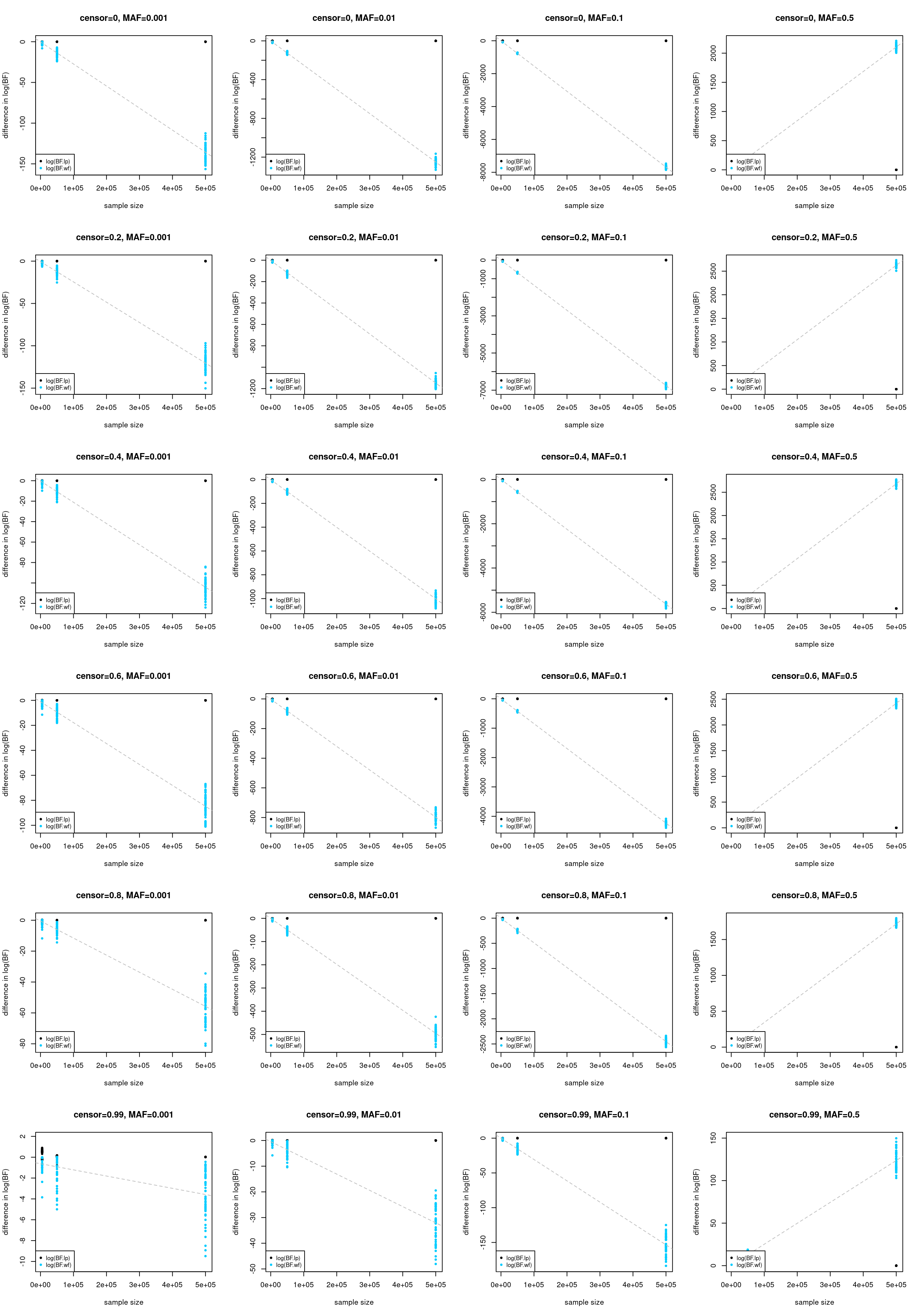
Compare different types of Bayes factor under different levels of censoring, minor allele frequency, effect size and sample size.

censoring = 0.00, 0.20, 0.40, 0.60, 0.80, 0.99
MAF = 0.001, 0.01, 0.1
n = 5000, 50000, 500000
b1 = -1， -0.1, -0.01, 0.01, 0.1, 1
BFs:

Numerical BF using Gaussian quadrature, our gold standard. https://yunqiyang0215.github.io/survival-susie/gauss_quad.html
Laplace-MLE BF
Wakefeld BF
Wakefeld BF with zscore from coxph() corrected by saddle point approximation. https://yunqiyang0215.github.io/survival-susie/SPAcox.html

library(latex2exp)

res = readRDS("/project2/mstephens/yunqiyang/surv-susie/sim202406/bf_comparison0712/res_bf.rds")
dat_list = lapply(1:length(res$DSC), function(x) res$compute_bf.result[[x]])
dat = do.call(rbind, dat_list)
dat2 = cbind(res$simulate.censor_lvl, res$simulate.allele_freq, res$simulate.n, 
             res$simulate.b1, dat)
colnames(dat2)[1:4] = c("censor_lvl", "allele_freq", "n", "b1")
dat2 = as.data.frame(dat2)

censor_lvl = unique(res$simulate.censor_lvl)
af = unique(res$simulate.allele_freq)
print(censor_lvl)

[1] 0.00 0.20 0.40 0.60 0.80 0.99

print(af)

[1] 0.001 0.010 0.100 0.500

1.1 Plot BF difference

par(mfrow = c(6,4))
for (i in 1:length(censor_lvl)){
  for (j in 1:length(af)){
    indx = which(dat2$censor_lvl == censor_lvl[i] & dat2$allele_freq == af[j] & dat2$b1 == 1)
    diff1 = dat2$lbf.numerical - dat2$lbf.laplace
    diff2 = dat2$lbf.numerical - dat2$lbf.wakefeld
    ymin = min(diff1[indx], diff2[indx]) - 1
    ymax = max(diff1[indx], diff2[indx]) + 1
    plot(dat2$n[indx], diff1[indx], ylim = c(ymin, ymax),
         main = paste0("censor=",censor_lvl[i], ", MAF=", af[j]),
         xlab = "sample size", ylab = "difference in log(BF)", cex = 0.8, pch = 20)
    points(dat2$n[indx], diff2[indx], col = "#00CCFF", cex = 0.8, pch = 20)
    fit = lm(diff2[indx] ~ dat2$n[indx])
    abline(fit, col = "grey", lty = 2) 
    legend("bottomleft", legend = c("log(BF.lp)", 'log(BF.wf)'), col = c(1, "#00CCFF"), pch = 20, cex = 0.8)
  }
}

Version	Author	Date
c219afc	yunqi yang	2024-10-11

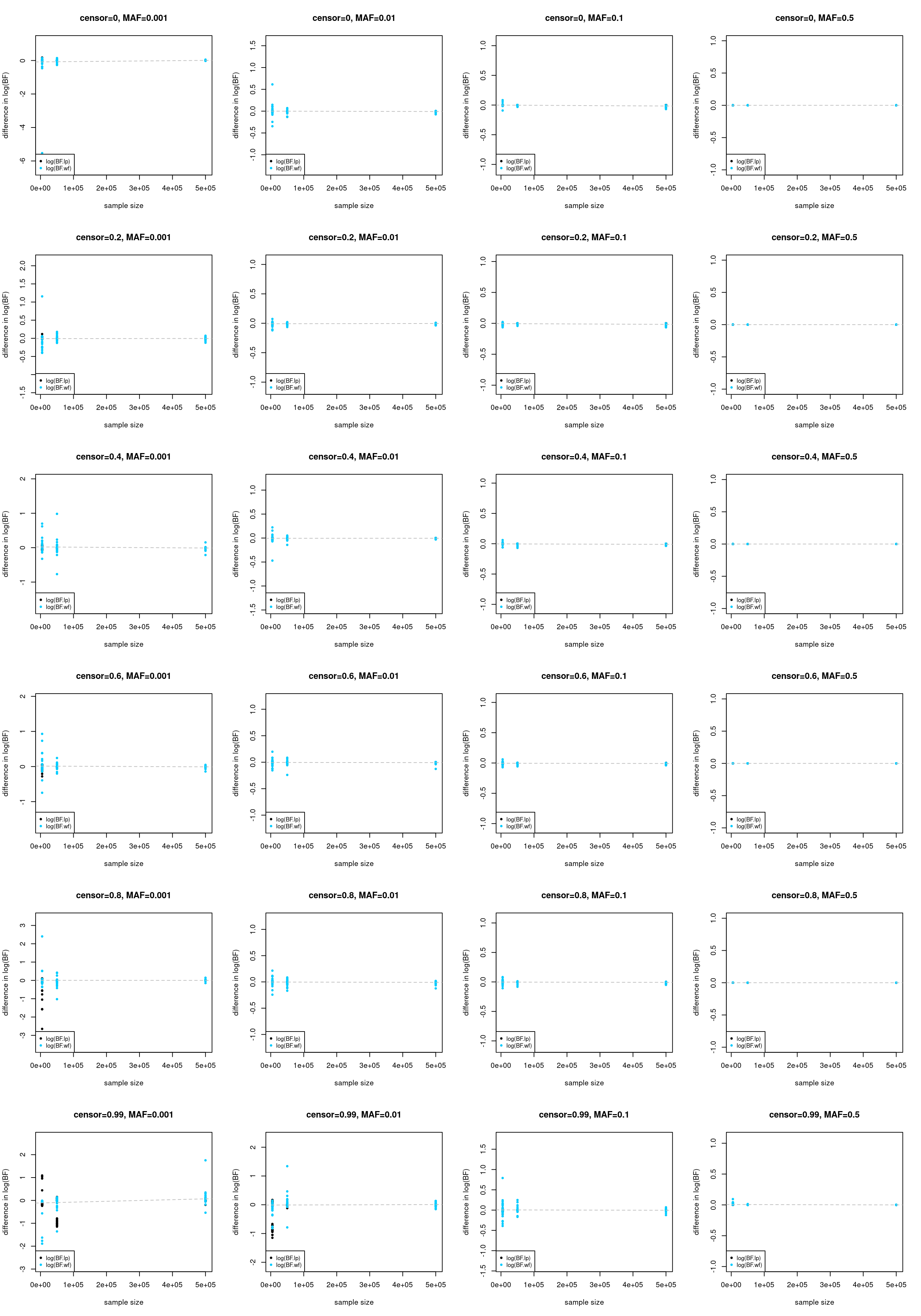
par(mfrow = c(6,4))
for (i in 1:length(censor_lvl)){
  for (j in 1:length(af)){
    indx = which(dat2$censor_lvl == censor_lvl[i] & dat2$allele_freq == af[j] & dat2$b1 == 0.01)
    diff1 = dat2$lbf.numerical - dat2$lbf.laplace
    diff2 = dat2$lbf.numerical - dat2$lbf.wakefeld
    ymin = min(diff1[indx], diff2[indx]) - 1
    ymax = max(diff1[indx], diff2[indx]) + 1
    plot(dat2$n[indx], diff1[indx], ylim = c(ymin, ymax),
         main = paste0("censor=",censor_lvl[i], ", MAF=", af[j]),
         xlab = "sample size", ylab = "difference in log(BF)", cex = 0.8, pch = 20)
    points(dat2$n[indx], diff2[indx], col = "#00CCFF", cex = 0.8, pch = 20)
    fit = lm(diff2[indx] ~ dat2$n[indx])
    abline(fit, col = "grey", lty = 2) 
    legend("bottomleft", legend = c("log(BF.lp)", 'log(BF.wf)'), col = c(1, "#00CCFF"), pch = 20, cex = 0.8)
  }
}

Version	Author	Date
c219afc	yunqi yang	2024-10-11

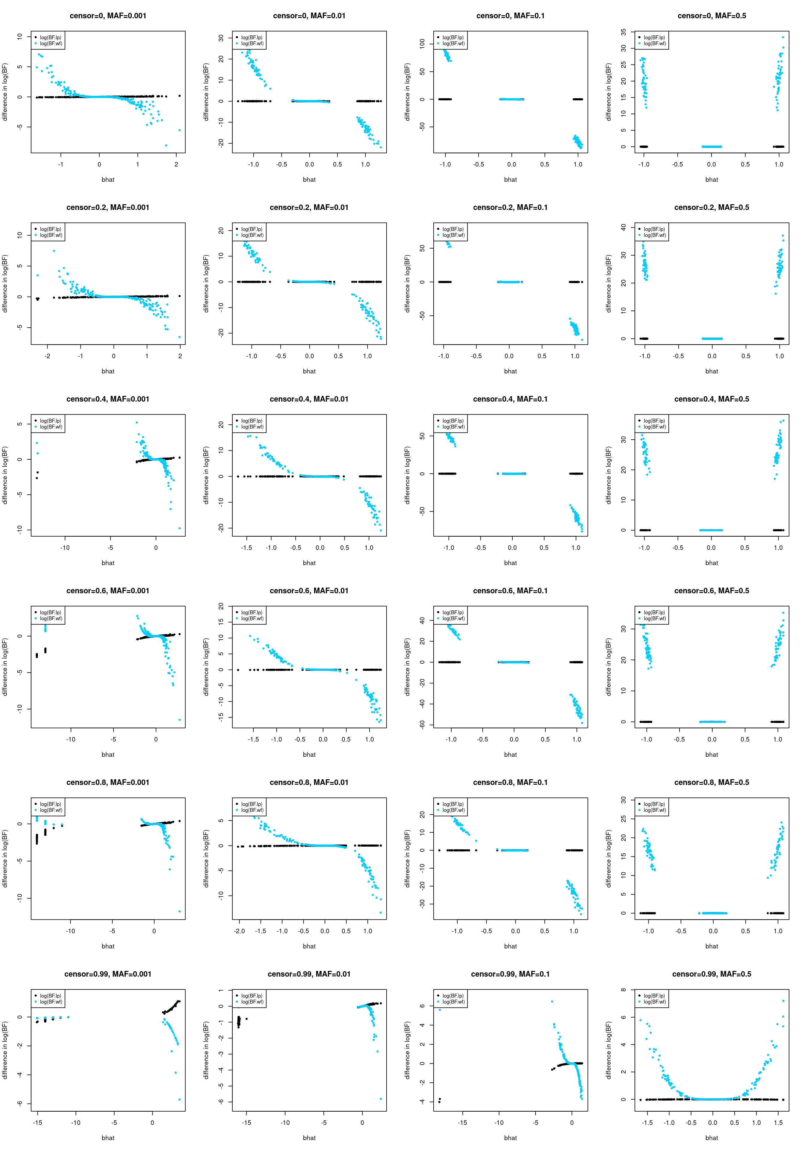
# Sample size small 
par(mfrow = c(6,4))
for (i in 1:length(censor_lvl)){
  for (j in 1:length(af)){
    indx = which(dat2$censor_lvl == censor_lvl[i] & dat2$allele_freq == af[j] & dat2$n == 5e3)
    diff1 = dat2$lbf.numerical - dat2$lbf.laplace
    diff2 = dat2$lbf.numerical - dat2$lbf.wakefeld
    ymin = min(diff1[indx], diff2[indx]) - 0.5
    ymax = max(diff1[indx], diff2[indx]) + 0.5
    plot(dat2$bhat[indx], diff1[indx], ylim = c(ymin, ymax), xlab = "bhat", ylab = "difference in log(BF)",
         main = paste0("censor=",censor_lvl[i], ", MAF=", af[j]), cex = 0.8, pch = 20)
    points(dat2$bhat[indx], diff2[indx], col = "#00CCFF", cex = 0.8, pch = 20)
    legend("topleft", legend = c("log(BF.lp)", 'log(BF.wf)'), col = c(1, "#00CCFF"), pch = 20, cex = 0.8)
  }
}

Version	Author	Date
c219afc	yunqi yang	2024-10-11

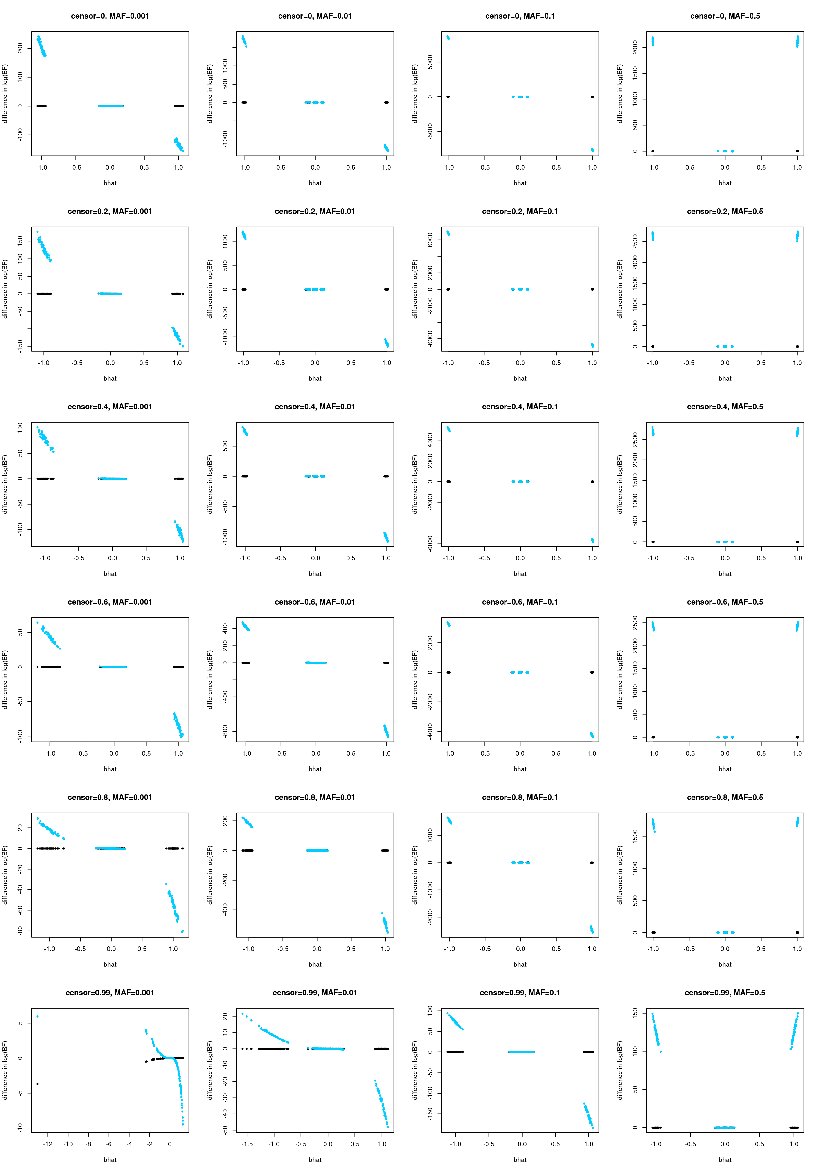
# Large n
par(mfrow = c(6,4))
for (i in 1:length(censor_lvl)){
  for (j in 1:length(af)){
    indx = which(dat2$censor_lvl == censor_lvl[i] & dat2$allele_freq == af[j] & dat2$n == 5e5)
    diff1 = dat2$lbf.numerical - dat2$lbf.laplace
    diff2 = dat2$lbf.numerical - dat2$lbf.wakefeld
    ymin = min(diff1[indx], diff2[indx]) - 0.5
    ymax = max(diff1[indx], diff2[indx]) + 0.5
    plot(dat2$bhat[indx], diff1[indx], ylim = c(ymin, ymax), xlab = "bhat", ylab = "difference in log(BF)",
         main = paste0("censor=",censor_lvl[i], ", MAF=", af[j]), cex = 0.8, pch = 20)
    points(dat2$bhat[indx], diff2[indx], col = "#00CCFF", cex = 0.8, pch = 20)
    #legend("topright", legend = c("log(BF.lp)", 'log(BF.wf)'), col = c(1, "#00CCFF"), pch = 20, cex = 0.8)
  }
}

Version	Author	Date
c219afc	yunqi yang	2024-10-11
8a1ddda	yunqi yang	2024-10-07

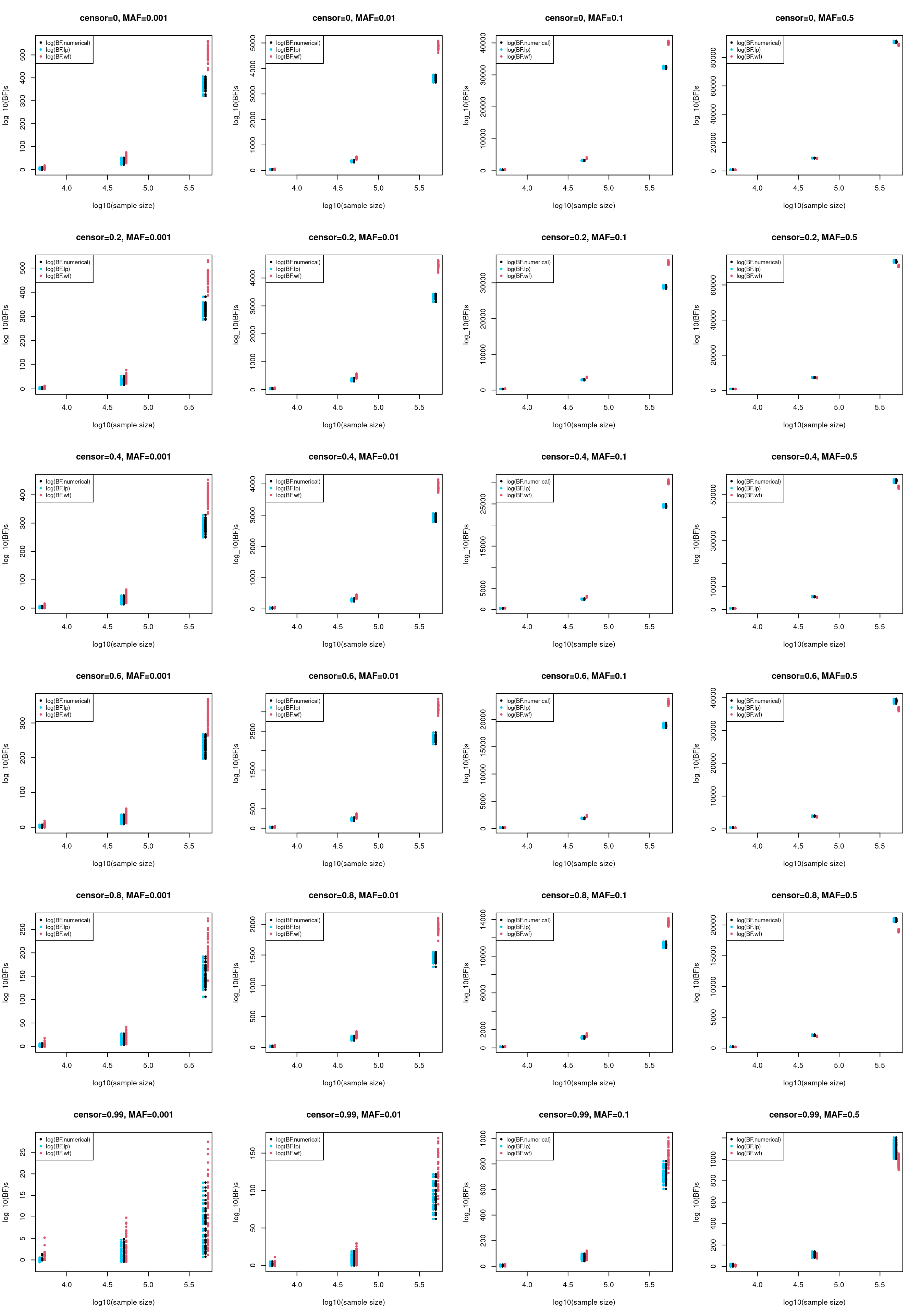
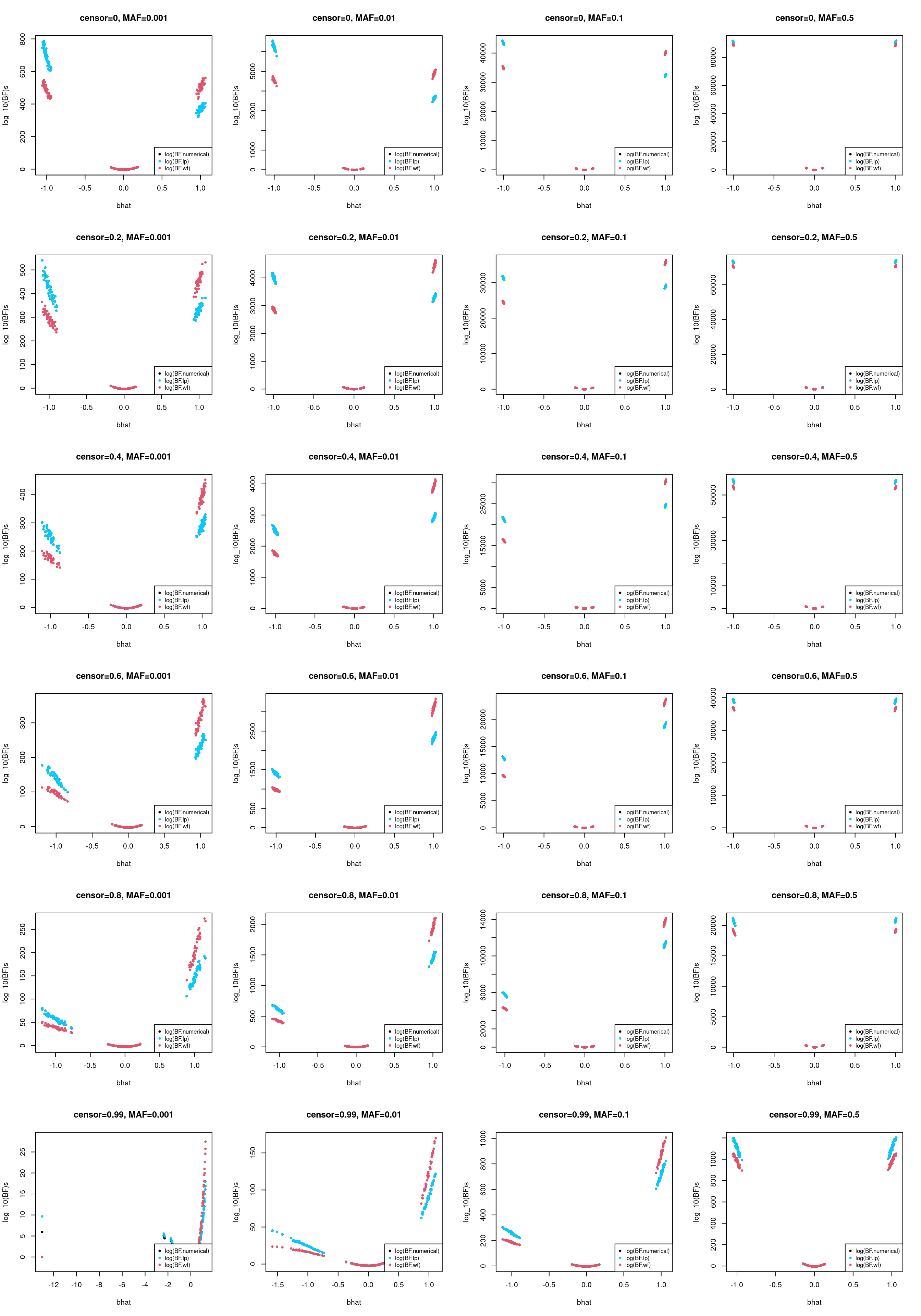
1.2 Plot different BFs across N/bhat

# Setting: b1 = 1
par(mfrow = c(6,4))
for (i in 1:length(censor_lvl)){
  for (j in 1:length(af)){
    indx = which(dat2$censor_lvl == censor_lvl[i] & dat2$allele_freq == af[j] & dat2$b1 == 1)
    ymin = min(dat2$lbf.numerical[indx], dat2$lbf.laplace[indx], dat2$lbf.wakefeld[indx]) - 1
    ymax = max(dat2$lbf.numerical[indx], dat2$lbf.laplace[indx], dat2$lbf.wakefeld[indx]) + 1
    plot(log10(dat2$n[indx]), dat2$lbf.numerical[indx], ylim = c(ymin, ymax),
         main = paste0("censor=",censor_lvl[i], ", MAF=", af[j]),
         xlab = "log10(sample size)", ylab = "log_10(BF)s", cex = 0.8, pch = 20)
    points(log10(dat2$n[indx])-0.03, dat2$lbf.laplace[indx], col = "#00CCFF", cex = 0.8, pch = 20)
    points(log10(dat2$n[indx])+0.03, dat2$lbf.wakefeld[indx], col = 2, cex = 0.8, pch = 20)
    legend("topleft", legend = c("log(BF.numerical)", "log(BF.lp)", 'log(BF.wf)'), col = c(1, "#00CCFF", 2), pch = 20, cex = 0.8)
  }
}

Version	Author	Date
c219afc	yunqi yang	2024-10-11
8a1ddda	yunqi yang	2024-10-07

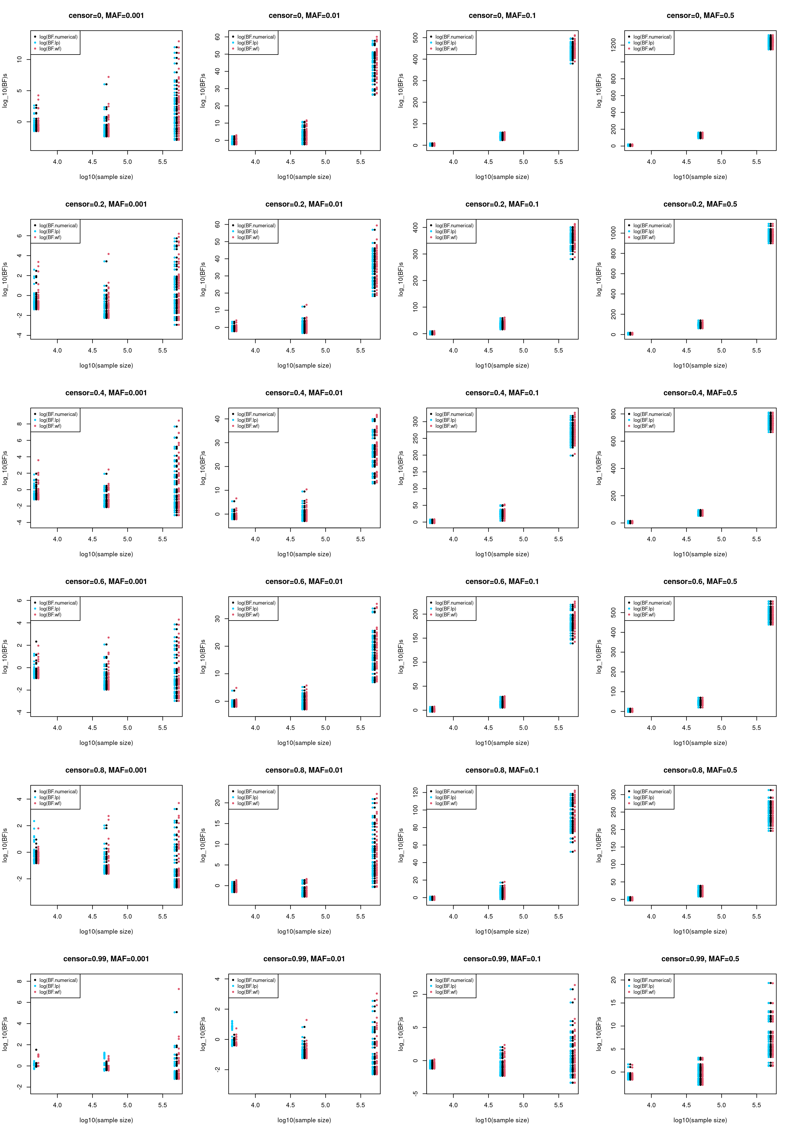
# Setting: b1 = 0.1
par(mfrow = c(6,4))
for (i in 1:length(censor_lvl)){
  for (j in 1:length(af)){
    indx = which(dat2$censor_lvl == censor_lvl[i] & dat2$allele_freq == af[j] & dat2$b1 == 0.1)
    ymin = min(dat2$lbf.numerical[indx], dat2$lbf.laplace[indx], dat2$lbf.wakefeld[indx]) - 1
    ymax = max(dat2$lbf.numerical[indx], dat2$lbf.laplace[indx], dat2$lbf.wakefeld[indx]) + 1
    plot(log10(dat2$n[indx]), dat2$lbf.numerical[indx], ylim = c(ymin, ymax),
         main = paste0("censor=",censor_lvl[i], ", MAF=", af[j]),
         xlab = "log10(sample size)", ylab = "log_10(BF)s", cex = 0.8, pch = 20)
    points(log10(dat2$n[indx])-0.03, dat2$lbf.laplace[indx], col = "#00CCFF", cex = 0.8, pch = 20)
    points(log10(dat2$n[indx])+0.03, dat2$lbf.wakefeld[indx], col = 2, cex = 0.8, pch = 20)
    legend("topleft", legend = c("log(BF.numerical)", "log(BF.lp)", 'log(BF.wf)'), col = c(1, "#00CCFF", 2), pch = 20, cex = 0.8)
  }
}

Version	Author	Date
c219afc	yunqi yang	2024-10-11
8a1ddda	yunqi yang	2024-10-07

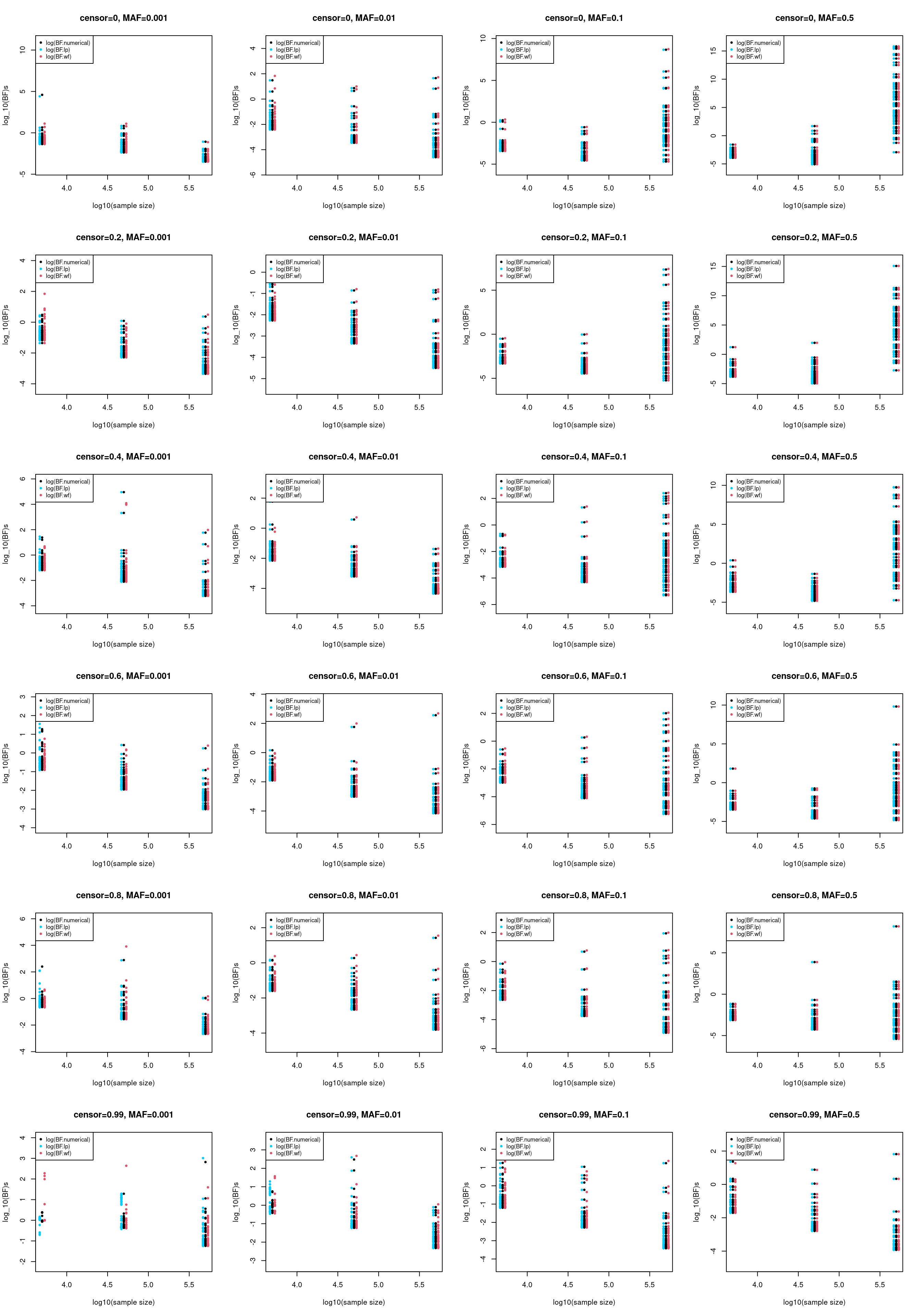
# Setting: b1 = 0.01
par(mfrow = c(6,4))
for (i in 1:length(censor_lvl)){
  for (j in 1:length(af)){
    indx = which(dat2$censor_lvl == censor_lvl[i] & dat2$allele_freq == af[j] & dat2$b1 == 0.01)
    ymin = min(dat2$lbf.numerical[indx], dat2$lbf.laplace[indx], dat2$lbf.wakefeld[indx]) - 1
    ymax = max(dat2$lbf.numerical[indx], dat2$lbf.laplace[indx], dat2$lbf.wakefeld[indx]) + 1
    plot(log10(dat2$n[indx]), dat2$lbf.numerical[indx], ylim = c(ymin, ymax),
         main = paste0("censor=",censor_lvl[i], ", MAF=", af[j]),
         xlab = "log10(sample size)", ylab = "log_10(BF)s", cex = 0.8, pch = 20)
    points(log10(dat2$n[indx])-0.03, dat2$lbf.laplace[indx], col = "#00CCFF", cex = 0.8, pch = 20)
    points(log10(dat2$n[indx])+0.03, dat2$lbf.wakefeld[indx], col = 2, cex = 0.8, pch = 20)
    legend("topleft", legend = c("log(BF.numerical)", "log(BF.lp)", 'log(BF.wf)'), col = c(1, "#00CCFF", 2), pch = 20, cex = 0.8)
  }
}

Version	Author	Date
c219afc	yunqi yang	2024-10-11
8a1ddda	yunqi yang	2024-10-07

# Sample size small 
par(mfrow = c(6,4))
for (i in 1:length(censor_lvl)){
  for (j in 1:length(af)){
    indx = which(dat2$censor_lvl == censor_lvl[i] & dat2$allele_freq == af[j] & dat2$n == 5e3)
    ymin = min(dat2$lbf.numerical[indx], dat2$lbf.laplace[indx], dat2$lbf.wakefeld[indx]) - 1
    ymax = max(dat2$lbf.numerical[indx], dat2$lbf.laplace[indx], dat2$lbf.wakefeld[indx]) + 1
    plot(dat2$bhat[indx], dat2$lbf.numerical[indx], ylim = c(ymin, ymax),
         main = paste0("censor=",censor_lvl[i], ", MAF=", af[j]),
         xlab = "bhat", ylab = "log_10(BF)s", cex = 0.8, pch = 20)
    points(dat2$bhat[indx], dat2$lbf.laplace[indx], col = "#00CCFF", cex = 0.8, pch = 20)
    points(dat2$bhat[indx], dat2$lbf.wakefeld[indx], col = 2, cex = 0.8, pch = 20)
    legend("bottomright", legend = c("log(BF.numerical)", "log(BF.lp)", 'log(BF.wf)'), col = c(1, "#00CCFF", 2), pch = 20, cex = 0.8)
  }
}

Version	Author	Date
410628d	yunqi yang	2024-10-11
c219afc	yunqi yang	2024-10-11

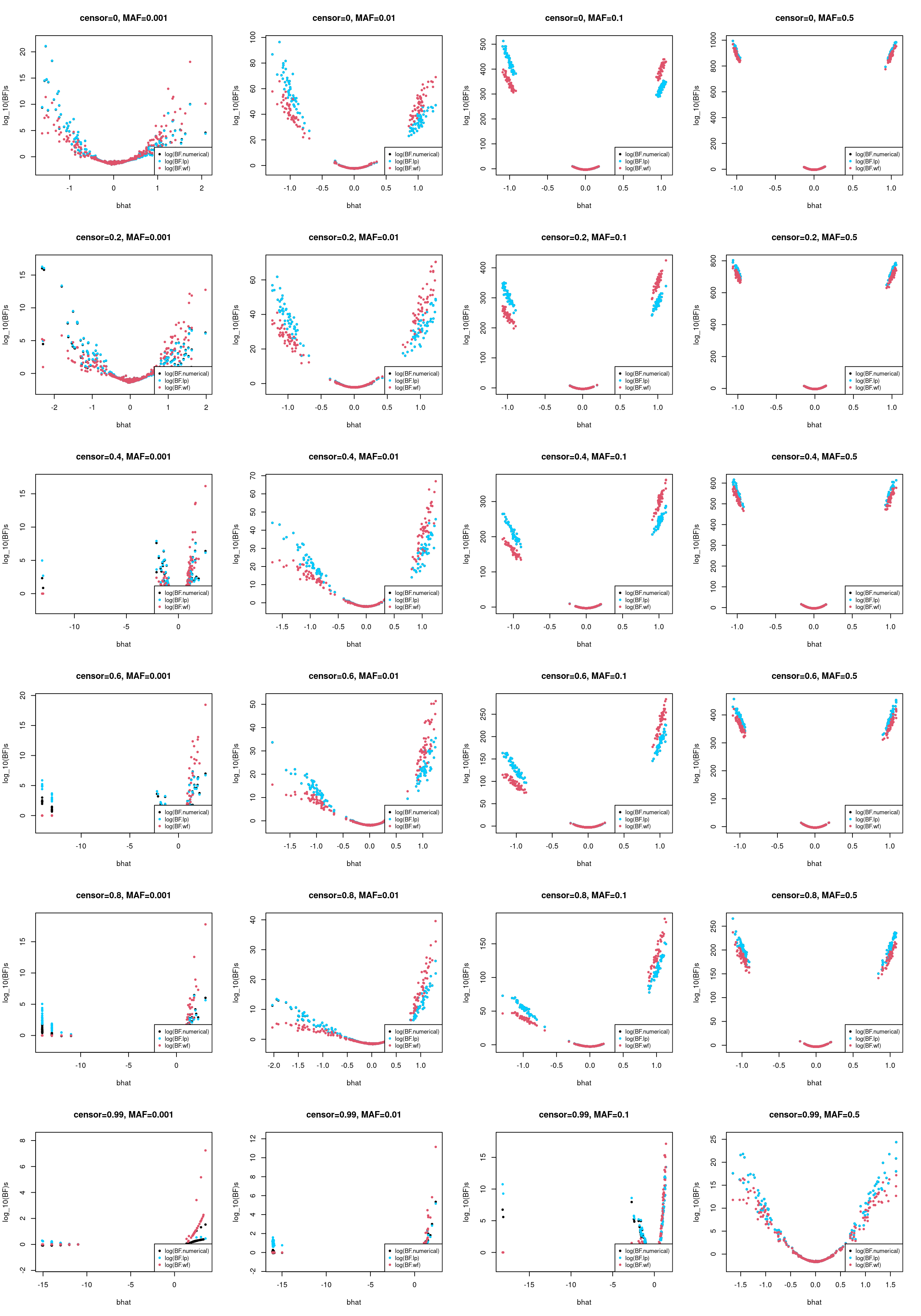
# Large n
par(mfrow = c(6,4))
for (i in 1:length(censor_lvl)){
  for (j in 1:length(af)){
    indx = which(dat2$censor_lvl == censor_lvl[i] & dat2$allele_freq == af[j] & dat2$n == 5e5)
    ymin = min(dat2$lbf.numerical[indx], dat2$lbf.laplace[indx], dat2$lbf.wakefeld[indx]) - 1
    ymax = max(dat2$lbf.numerical[indx], dat2$lbf.laplace[indx], dat2$lbf.wakefeld[indx]) + 1
    plot(dat2$bhat[indx], dat2$lbf.numerical[indx], ylim = c(ymin, ymax),
         main = paste0("censor=",censor_lvl[i], ", MAF=", af[j]),
         xlab = "bhat", ylab = "log_10(BF)s", cex = 0.8, pch = 20)
    points(dat2$bhat[indx], dat2$lbf.laplace[indx], col = "#00CCFF", cex = 0.8, pch = 20)
    points(dat2$bhat[indx], dat2$lbf.wakefeld[indx], col = 2, cex = 0.8, pch = 20)
    legend("bottomright", legend = c("log(BF.numerical)", "log(BF.lp)", 'log(BF.wf)'), col = c(1, "#00CCFF", 2), pch = 20, cex = 0.8)
  }
}

Version	Author	Date
410628d	yunqi yang	2024-10-11
c219afc	yunqi yang	2024-10-11

1.3 Plot numerical BF against wakefield/laplace BF

pdf("/project2/mstephens/yunqiyang/surv-susie/survival-susie/output/bf_comparison_b_1_n_500000.pdf", width = 8, height = 12)
par(mfrow = c(4,3))
censor_lvl <- c(0, 0.4, 0.8, 0.99)
af <- c(0.001, 0.010, 0.100)
for (i in 1:length(censor_lvl)){
  for (j in 1:length(af)){
    indx = which(res$simulate.censor_lvl == censor_lvl[i] & res$simulate.allele_freq == af[j]
                 & res$simulate.n == 5e5 & res$simulate.b1 == 1)
    dat = t(sapply(indx, function(x) res$compute_bf.result[[x]]))
    plot(x = dat[, 'lbf.numerical'], y = dat[, 'lbf.laplace'], pch = 20, main = paste0("censor=",censor_lvl[i], ", MAF=", af[j]),
         ylim = c(min(dat[,c(4:6)])-1, max(dat[, c(4:6)])+1), cex = 0.8, col = "blue",
         xlab = TeX("$log_{10}$(BF numerical)"), ylab = TeX("$log_{10}$($BF_{LM}$)"))
    abline(a = 0, b = 1, col = "grey")
    #legend("topleft", legend = c(TeX("$log_{10}$(BF.lp)"), TeX("$log_{10}$(BF.wf)")), col = c(1, "#26B300"), pch = 20, cex = 0.8)
  }
}

pdf("/project2/mstephens/yunqiyang/surv-susie/survival-susie/output/bf_comparison_b_0.1_n_500000.pdf", width = 8, height = 12)
par(mfrow = c(4,3))
censor_lvl <- c(0, 0.4, 0.8, 0.99)
af <- c(0.001, 0.010, 0.100)
for (i in 1:length(censor_lvl)){
  for (j in 1:length(af)){
    indx = which(res$simulate.censor_lvl == censor_lvl[i] & res$simulate.allele_freq == af[j]
                 & res$simulate.n == 5e5 & res$simulate.b1 == 0.1)
    dat = t(sapply(indx, function(x) res$compute_bf.result[[x]]))
    plot(x = dat[, 'lbf.numerical'], y = dat[, 'lbf.laplace'], pch = 20, main = paste0("censor=",censor_lvl[i], ", MAF=", af[j]),
         ylim = c(min(dat[,c(4:6)])-1, max(dat[, c(4:6)])+1), cex = 0.8,
         xlab = TeX("$log_{10}(BF^{GH})$"), ylab = TeX("Other $log_{10}$(BFs)"))
    points(dat[, 'lbf.numerical'], dat[,'lbf.wakefeld'], col = "#26B300", pch = 20, cex = 0.8)
    abline(a = 0, b = 1, col = "grey")
    legend("topleft", legend = c(TeX("$log_{10}(\\hat{BF})$"), TeX("$log_{10}(ABF)$")), col = c(1, "#26B300"), pch = 20, cex = 0.8)
  }
}

pdf("/project2/mstephens/yunqiyang/surv-susie/survival-susie/output/bf_comparison_b_0.01_n_500000.pdf", width = 8, height = 18)
par(mfrow = c(6,3))

for (i in 1:length(censor_lvl)){
  for (j in 1:length(af)){
    indx = which(res$simulate.censor_lvl == censor_lvl[i] & res$simulate.allele_freq == af[j]
                 & res$simulate.n == 5e5 & res$simulate.b1 == 0.01)
    dat = t(sapply(indx, function(x) res$compute_bf.result[[x]]))
    plot(x = dat[, 'lbf.numerical'], y = dat[, 'lbf.laplace'], pch = 20, main = paste0("censor=",censor_lvl[i], ", MAF=", af[j]),
         ylim = c(min(dat[,c(4:6)])-1, max(dat[,c(4:6)])+1), cex = 0.8,
         xlab = TeX("$log_{10}(BF^{GH})$"), ylab = TeX("Other $log_{10}$(BFs)"))
    points(dat[, 'lbf.numerical'], dat[,'lbf.wakefeld'], col = "#26B300", pch = 20, cex = 0.8)
    abline(a = 0, b = 1, col = "grey")
    legend("topleft", legend = c(TeX("$log_{10}(BF^L)$"), TeX("$log_{10}(BF^W)$")), col = c(1, "#26B300"), pch = 20, cex = 0.8)
  }
}

1. Check BF

dat.sub = dat2[dat2$censor_lvl == 0 & dat2$n == 5e5 & dat2$allele_freq == 0.1, ]

par(mfrow = c(2,2))
hist(dat.sub$zscore[dat.sub$b1 == -1], xlab = "zscore", main = "true b = -1; MAF = 0.1; n = 5e5; no censor")
hist(dat.sub$zscore[dat.sub$b1 == 1],  xlab = "zscore", main = "true b = 1; MAF = 0.1; n = 5e5; no censor")
hist(dat.sub$bhat[dat.sub$b1 == -1], xlab = "bhat", main = "true b = -1; MAF = 0.1; n = 5e5; no censor")
hist(dat.sub$bhat[dat.sub$b1 == 1], xlab = "bhat", main = "true b = 1; MAF = 0.1; n = 5e5; no censor")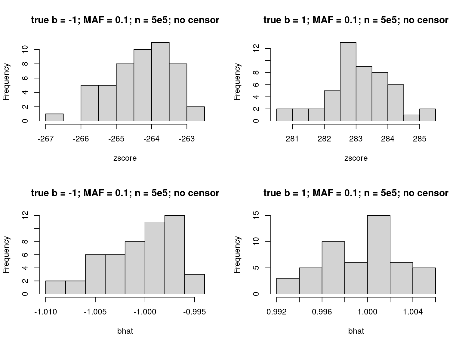

Version	Author	Date
c219afc	yunqi yang	2024-10-11
8a1ddda	yunqi yang	2024-10-07
6445624	yunqi yang	2024-09-18
5b1f3bf	yunqi yang	2024-09-15
546c2bf	yunqi yang	2024-08-26

par(mfrow = c(2,2))
hist(dat.sub$lbf.numerical[dat.sub$b1 == -1],  xlab = "log(BF.numerical)", main = "true b = -1; MAF = 0.1; n = 5e5; no censor")
hist(dat.sub$lbf.numerical[dat.sub$b1 == 1],  xlab = "log(BF.numerical)", main = "true b = 1; MAF = 0.1; n = 5e5; no censor")
hist(dat.sub$lbf.wakefeld[dat.sub$b1 == -1],  xlab = "log(BF.wakefield)", main = "true b = -1; MAF = 0.1; n = 5e5; no censor")
hist(dat.sub$lbf.wakefeld[dat.sub$b1 == 1],  xlab = "log(BF.wakefield)", main = "true b = 1; MAF = 0.1; n = 5e5; no censor")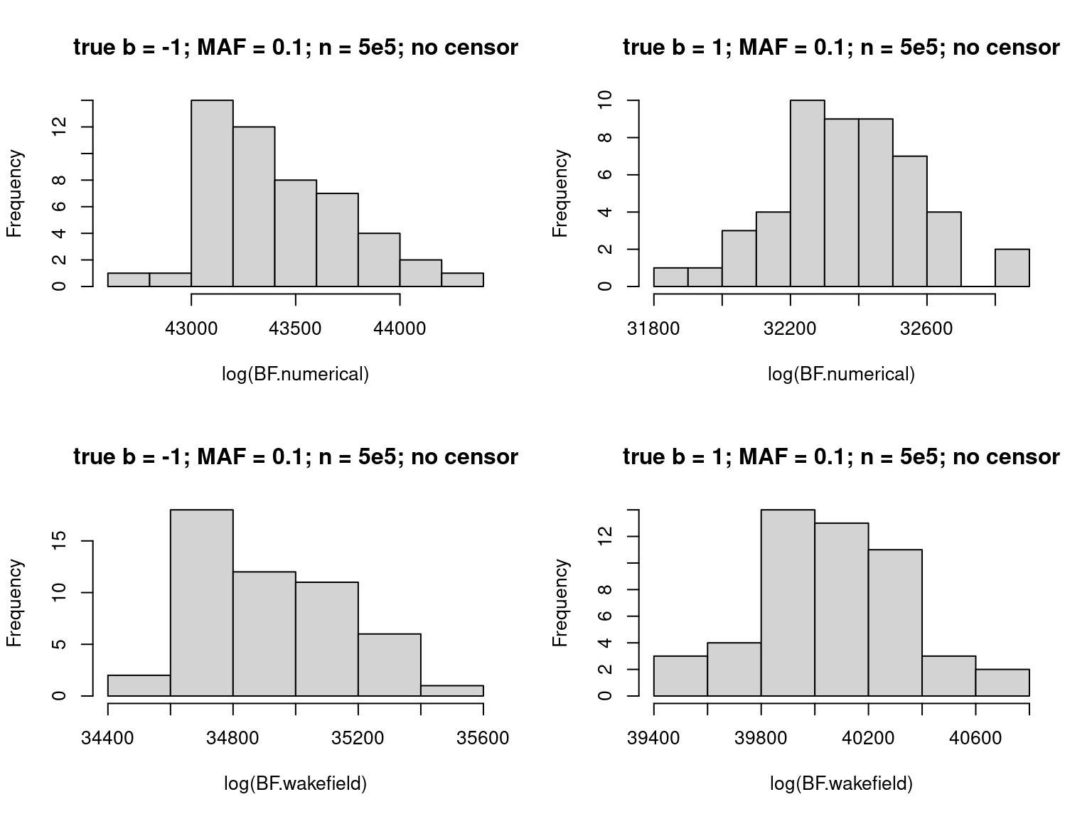

Version	Author	Date
c219afc	yunqi yang	2024-10-11
8a1ddda	yunqi yang	2024-10-07
6445624	yunqi yang	2024-09-18
5b1f3bf	yunqi yang	2024-09-15
546c2bf	yunqi yang	2024-08-26

2. Check BF when flip binary x.

I experimented with two different sample sizes, n = 5e3 and 5e5.

res = readRDS("/project2/mstephens/yunqiyang/surv-susie/sim202406/bf_comparison0825/res_bf.rds")

dat_list = lapply(1:length(res$DSC), function(x) res$compute_bf.result[[x]])
dat = do.call(rbind, dat_list)
dat2 = cbind(res$simulate.allele_freq, res$simulate.n, res$simulate.b1, dat)
colnames(dat2)[1:3] = c("allele_freq", "n", "b1")
dat2 = as.data.frame(dat2)
dat2$flip = res$compute_bf.flip

1. n = 5e3

par(mfrow = c(2,2))
n = 5e3
plot(dat2$zscore[dat2$n == n & dat2$flip == "flip"], dat2$zscore[dat2$n == n & dat2$flip == "nonflip"],
     xlim = c(-23,-18), ylim = c(18, 23), main = "zscore", xlab = "x flipped", ylab = "x original")
abline(a = 0, b = -1, col = "red")

plot(dat2$bhat[dat2$n == n & dat2$flip == "flip"], dat2$bhat[dat2$n == n & dat2$flip == "nonflip"], main = "bhat",
     xlab = "x flipped", ylab = "x original")
abline(a = 0, b = -1, col = "red")

plot(dat2$lbf.wakefeld[dat2$n == n & dat2$flip == "flip"], dat2$lbf.wakefeld[dat2$n == n & dat2$flip == "nonflip"], main = "Wakefield log(BF)", xlab = "x flipped", ylab = "x original")
abline(a = 0, b = 1, col = "red")

plot(dat2$lbf.numerical[dat2$n == n & dat2$flip == "flip"], dat2$lbf.numerical[dat2$n == n & dat2$flip == "nonflip"], main = "Numerical log(BF)", xlab = "x flipped", ylab = "x original")
abline(a = 0, b = 1, col = "red")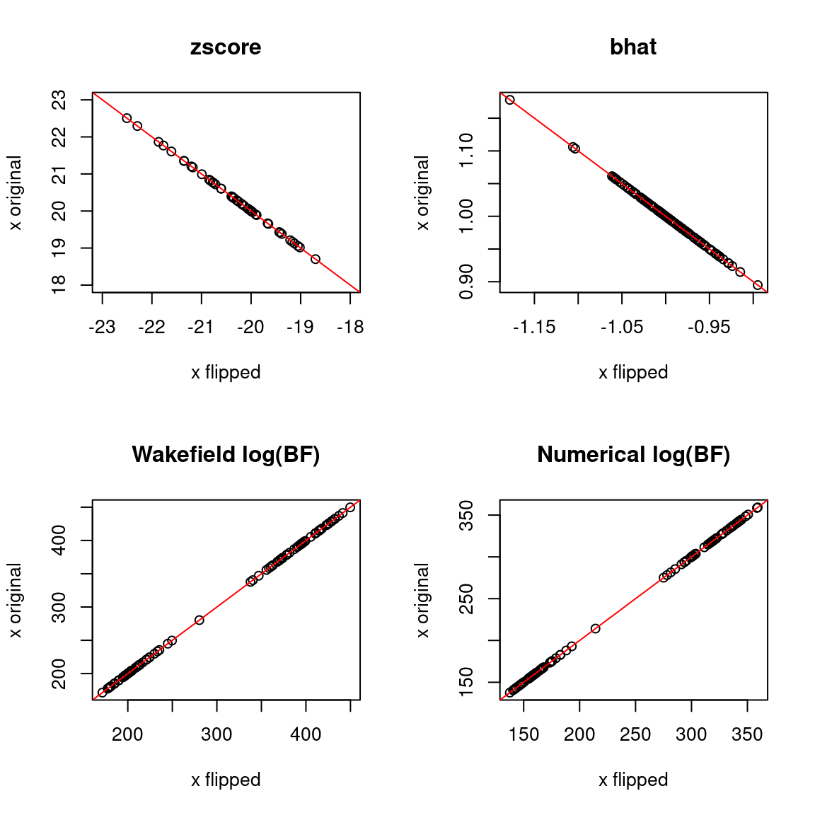

Version	Author	Date
c219afc	yunqi yang	2024-10-11
8a1ddda	yunqi yang	2024-10-07
6445624	yunqi yang	2024-09-18
5b1f3bf	yunqi yang	2024-09-15

plot(dat2$bhat[dat2$n == n], dat2$lbf.wakefeld[dat2$n == n]-dat2$lbf.numerical[dat2$n == n], xlab = "bhat", ylab = "log(BF.wakefield) - log(BF.numerical)")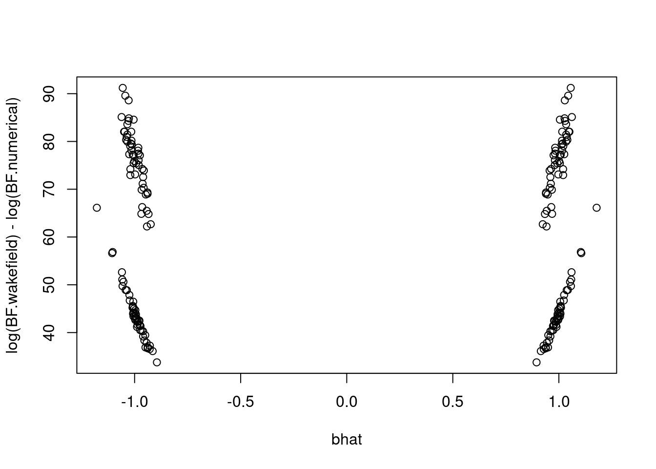

Version	Author	Date
c219afc	yunqi yang	2024-10-11
8a1ddda	yunqi yang	2024-10-07
6445624	yunqi yang	2024-09-18

2. n = 5e5

n = 5e5
plot(dat2$zscore[dat2$n == n & dat2$flip == "flip"], dat2$zscore[dat2$n == n & dat2$flip == "nonflip"],
     main = "zscore", xlab = "x flipped", ylab = "x original")
abline(a = 0, b = -1, col = "red")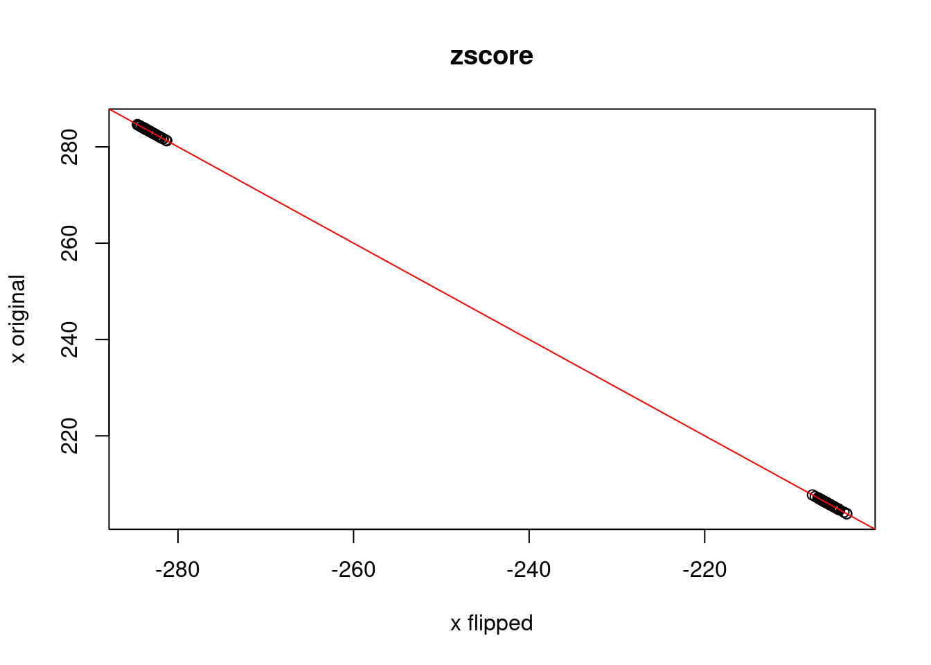

Version	Author	Date
c219afc	yunqi yang	2024-10-11
8a1ddda	yunqi yang	2024-10-07

plot(dat2$bhat[dat2$n == n & dat2$flip == "flip"], dat2$bhat[dat2$n == n & dat2$flip == "nonflip"], main = "bhat")
abline(a = 0, b = -1, col = "red", xlab = "x flipped", ylab = "x original")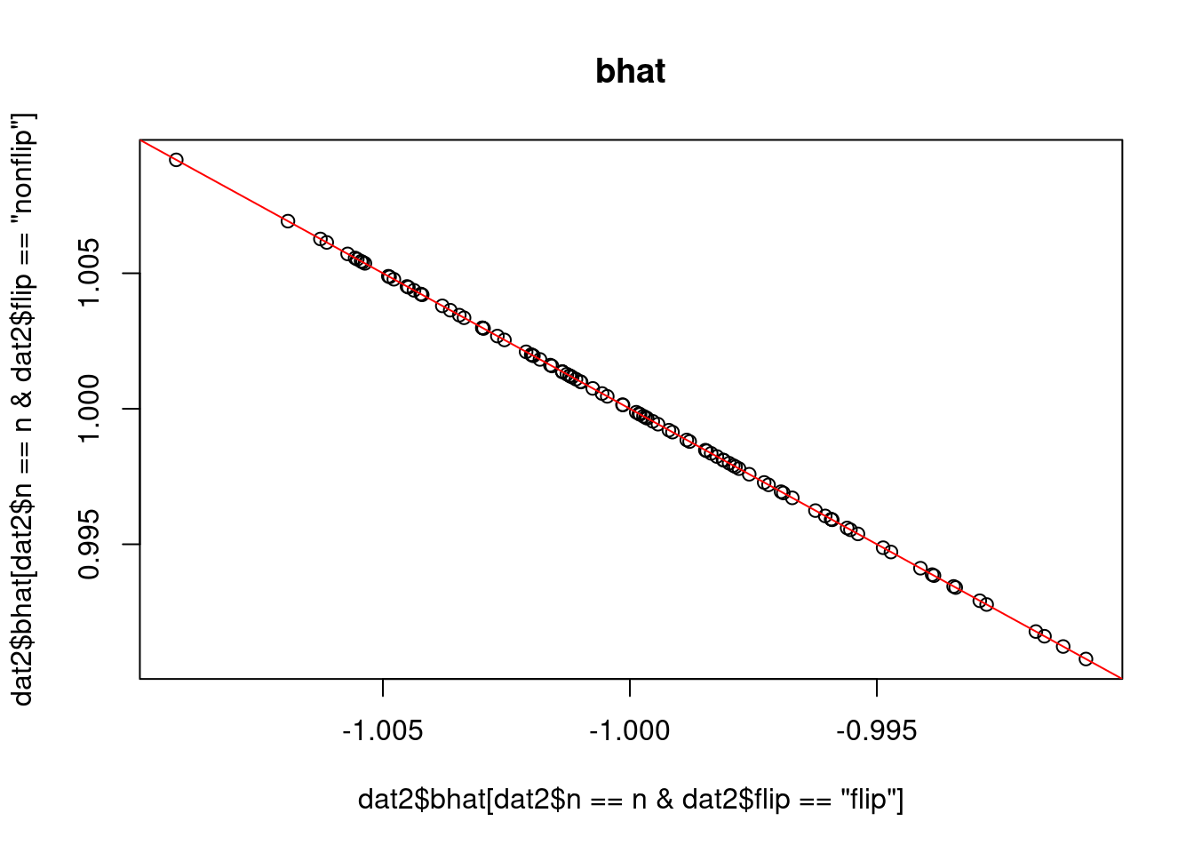

Version	Author	Date
c219afc	yunqi yang	2024-10-11

plot(dat2$lbf.wakefeld[dat2$n == n & dat2$flip == "flip"], dat2$lbf.wakefeld[dat2$n == n & dat2$flip == "nonflip"], main = "Wakefield log(BF)", xlab = "x flipped", ylab = "x original")
abline(a = 0, b = 1, col = "red")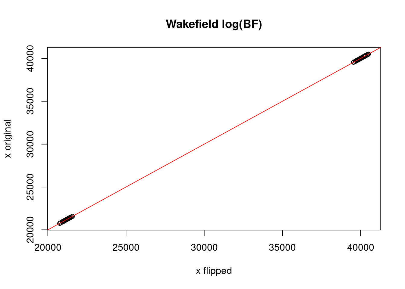

Version	Author	Date
c219afc	yunqi yang	2024-10-11

plot(dat2$lbf.numerical[dat2$n == n & dat2$flip == "flip"], dat2$lbf.numerical[dat2$n == n & dat2$flip == "nonflip"], main = "Numerical log(BF)", xlab = "x flipped", ylab = "x original")
abline(a = 0, b = 1, col = "red")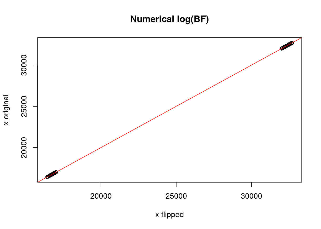

Version	Author	Date
c219afc	yunqi yang	2024-10-11

plot(dat2$bhat[dat2$n == n], dat2$lbf.wakefeld[dat2$n == n]-dat2$lbf.numerical[dat2$n == n], xlab = "bhat", ylab = "log(BF.wakefield) - log(BF.numerical)")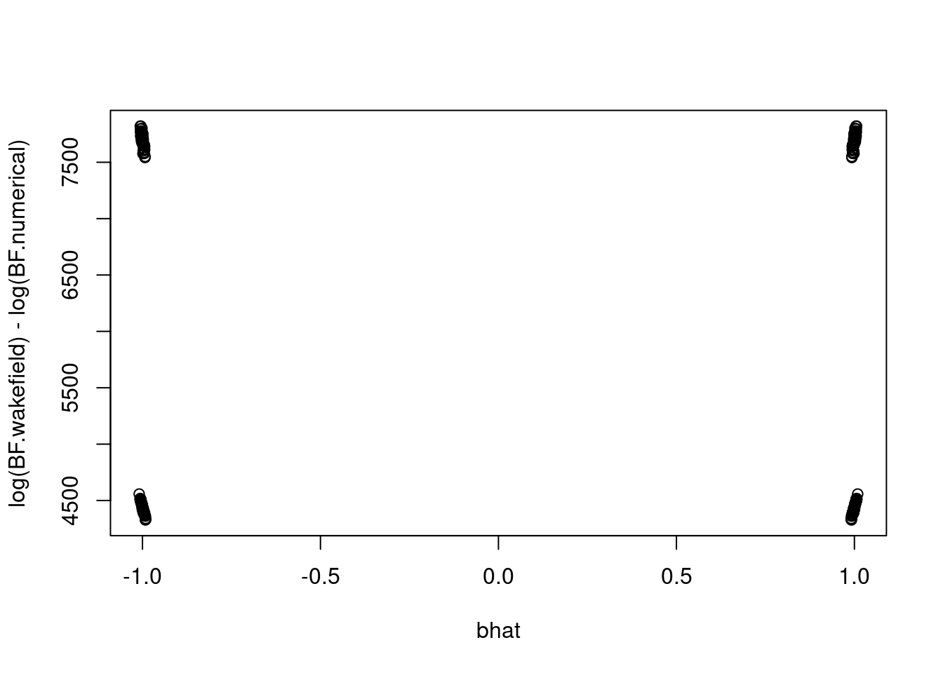

Version	Author	Date
c219afc	yunqi yang	2024-10-11

3. Computation time of Gauss-Hermite vs. laplace BF

par(mfrow = c(1,2))
hist(dat2$time.lp)
hist(dat2$time.gh)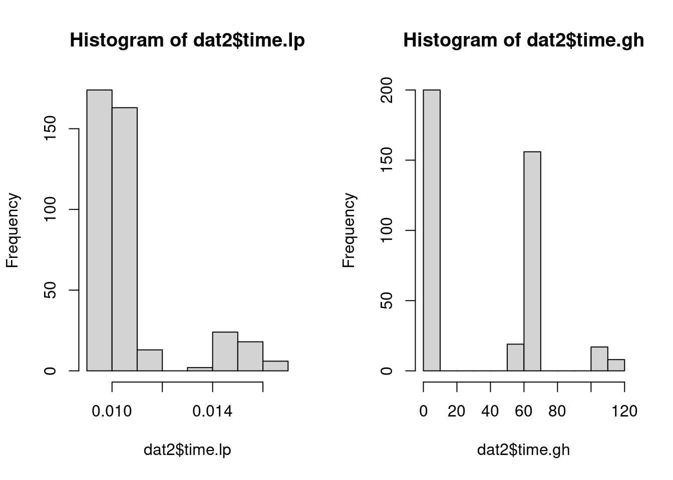

Version	Author	Date
c219afc	yunqi yang	2024-10-11

mean(dat2$time.lp)

[1] 0.0111275

mean(dat2$time.gh)

[1] 35.52377

sessionInfo()

R version 4.2.0 (2022-04-22)
Platform: x86_64-pc-linux-gnu (64-bit)
Running under: CentOS Linux 7 (Core)

Matrix products: default
BLAS/LAPACK: /software/openblas-0.3.13-el7-x86_64/lib/libopenblas_haswellp-r0.3.13.so

locale:
 [1] LC_CTYPE=en_US.UTF-8 LC_NUMERIC=C         LC_TIME=C           
 [4] LC_COLLATE=C         LC_MONETARY=C        LC_MESSAGES=C       
 [7] LC_PAPER=C           LC_NAME=C            LC_ADDRESS=C        
[10] LC_TELEPHONE=C       LC_MEASUREMENT=C     LC_IDENTIFICATION=C 

attached base packages:
[1] stats     graphics  grDevices utils     datasets  methods   base     

other attached packages:
[1] latex2exp_0.9.4 workflowr_1.7.0

loaded via a namespace (and not attached):
 [1] Rcpp_1.0.12      highr_0.9        compiler_4.2.0   pillar_1.9.0    
 [5] bslib_0.3.1      later_1.3.0      git2r_0.30.1     jquerylib_0.1.4 
 [9] tools_4.2.0      getPass_0.2-2    digest_0.6.29    jsonlite_1.8.0  
[13] evaluate_0.15    lifecycle_1.0.4  tibble_3.2.1     pkgconfig_2.0.3 
[17] rlang_1.1.3      cli_3.6.2        rstudioapi_0.13  yaml_2.3.5      
[21] xfun_0.30        fastmap_1.1.0    httr_1.4.3       stringr_1.5.1   
[25] knitr_1.39       fs_1.5.2         vctrs_0.6.5      sass_0.4.1      
[29] rprojroot_2.0.3  glue_1.6.2       R6_2.5.1         processx_3.8.0  
[33] fansi_1.0.3      rmarkdown_2.14   callr_3.7.3      magrittr_2.0.3  
[37] whisker_0.4      ps_1.7.0         promises_1.2.0.1 htmltools_0.5.2 
[41] httpuv_1.6.5     utf8_1.2.2       stringi_1.7.6