model_atac

workflowr

• Summary
• Checks
• Past versions

Last updated: 2020-08-18

Checks: 6 1

Knit directory: gene_level_fine_mapping/

This reproducible R Markdown analysis was created with workflowr (version 1.6.1). The Checks tab describes the reproducibility checks that were applied when the results were created. The Past versions tab lists the development history.

---

R Markdown file: up-to-date

Great! Since the R Markdown file has been committed to the Git repository, you know the exact version of the code that produced these results.

Environment: empty

Great job! The global environment was empty. Objects defined in the global environment can affect the analysis in your R Markdown file in unknown ways. For reproduciblity it’s best to always run the code in an empty environment.

Seed: set.seed(20200622)

The command set.seed(20200622) was run prior to running the code in the R Markdown file. Setting a seed ensures that any results that rely on randomness, e.g. subsampling or permutations, are reproducible.

Session information: recorded

Great job! Recording the operating system, R version, and package versions is critical for reproducibility.

Cache: none

Nice! There were no cached chunks for this analysis, so you can be confident that you successfully produced the results during this run.

File paths: absolute

Using absolute paths to the files within your workflowr project makes it difficult for you and others to run your code on a different machine. Change the absolute path(s) below to the suggested relative path(s) to make your code more reproducible.

absolute	relative
/Users/nicholeyang/Desktop/gene_level_fine_mapping/data/train_all.RData	data/train_all.RData

Repository version: 038b52c

Great! You are using Git for version control. Tracking code development and connecting the code version to the results is critical for reproducibility.

The results in this page were generated with repository version 038b52c. See the Past versions tab to see a history of the changes made to the R Markdown and HTML files.

Note that you need to be careful to ensure that all relevant files for the analysis have been committed to Git prior to generating the results (you can use wflow_publish or wflow_git_commit). workflowr only checks the R Markdown file, but you know if there are other scripts or data files that it depends on. Below is the status of the Git repository when the results were generated:

Ignored files:
    Ignored:    .DS_Store
    Ignored:    .Rhistory
    Ignored:    .Rproj.user/
    Ignored:    analysis/.DS_Store
    Ignored:    analysis/.RData
    Ignored:    analysis/.Rhistory

Untracked files:
    Untracked:  analysis/atac_eqtl.Rmd
    Untracked:  data/hic_eqtl.RData
    Untracked:  data/train_add_hic.RData
    Untracked:  data/train_all.RData

Unstaged changes:
    Modified:   analysis/add_hic_feature.Rmd

Note that any generated files, e.g. HTML, png, CSS, etc., are not included in this status report because it is ok for generated content to have uncommitted changes.

---

These are the previous versions of the repository in which changes were made to the R Markdown (analysis/model_atac.Rmd) and HTML (docs/model_atac.html) files. If you’ve configured a remote Git repository (see ?wflow_git_remote), click on the hyperlinks in the table below to view the files as they were in that past version.

File	Version	Author	Date	Message
Rmd	038b52c	yunqiyang0215	2020-08-18	wflow_publish(“analysis/model_atac.Rmd”)
html	a32fa5b	yunqiyang0215	2020-08-11	Build site.
Rmd	0e0f656	yunqiyang0215	2020-08-11	wflow_publish(“analysis/model_atac.Rmd”)

---

load('/Users/nicholeyang/Desktop/gene_level_fine_mapping/data/train_all.RData')

head(train_all_sig)

  gene_name      snp_loc38             variant_id UTR5 UTR3 exon intron
1      A1BG chr19:57866502 chr19_57866502_T_C_b38    0    0    0      0
2      A1BG chr19:58059544 chr19_58059544_T_G_b38    0    0    0      0
3      A1BG chr19:58170494 chr19_58170494_G_T_b38    0    0    0      0
4      A1BG chr19:58228973 chr19_58228973_T_G_b38    0    0    0      0
5      A1BG chr19:58330182 chr19_58330182_C_T_b38    0    0    0      0
6      A1BG chr19:58359927 chr19_58359927_G_A_b38    0    0    0      0
  upstream tss_dist_to_snp y Mon Mac0 Mac1 Mac2 Neu MK EP Ery FoeT nCD4 tCD4
1        0          481132 0   0    0    0    0   0  0  0   0    0    0    0
2        0          288090 0   0    0    0    0   0  0  0   0    0    0    0
3        0          177140 0   0    0    0    0   0  0  0   0    0    0    0
4        0          118661 0   0    0    0    0   0  0  0   0    0    0    0
5        0           17452 1   0    0    0    0   0  0  0   0    0    0    0
6        0            6428 1   0    0    0    0   0  0  0   0    0    0    0
  aCD4 naCD4 nCD8 tCD8 nB tB correlation
1    0     0    0    0  0  0           0
2    0     0    0    0  0  0           0
3    0     0    0    0  0  0           0
4    0     0    0    0  0  0           0
5    0     0    0    0  0  0           0
6    0     0    0    0  0  0           0

correlation by distance

Comment: ATAC features are mostly concentrated in the range < 5e5.

par(mfrow = c(1,2))
plot(train_all_sig$tss_dist_to_snp, train_all_sig$correlation, xlab = 'distance', ylab = 'correlation')

plot(train_all_sig[train_all_sig$correlation>0.4, ]$tss_dist_to_snp, train_all_sig[train_all_sig$correlation>0.4, ]$correlation, xlab = 'distance', ylab = 'correlation')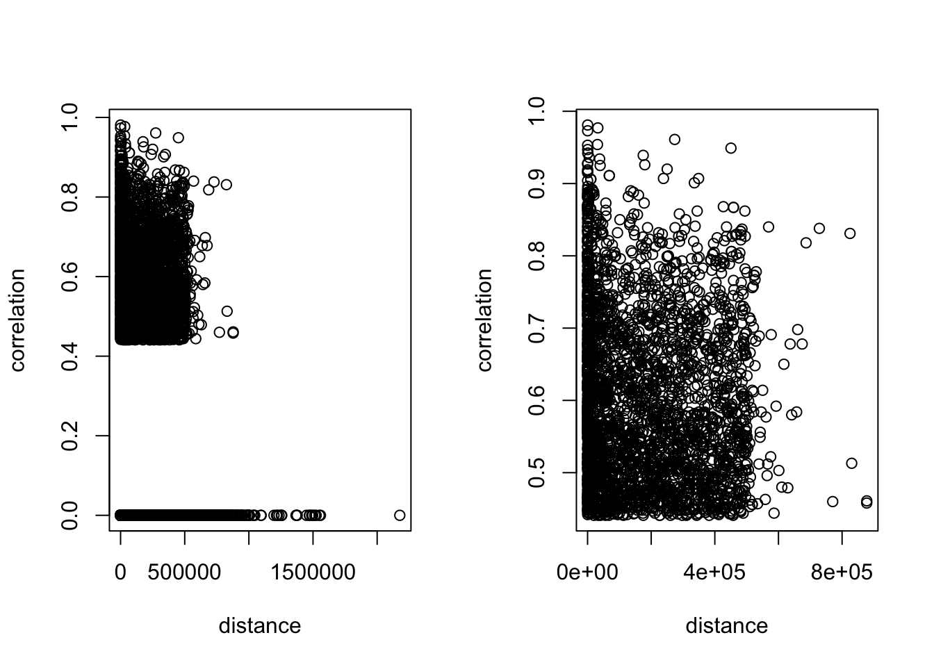

direct regress correlation on y

Complete separation?

https://courses.ms.ut.ee/MTMS.01.011/2018_spring/uploads/Main/GLM_slides_7_binary_response_ii.pdf

fit1 = glm(y ~ correlation, data = train_all_sig, family = "binomial")
fit2 = glm(y ~ correlation + tss_dist_to_snp, data = train_all_sig, family = "binomial")

Warning: glm.fit: fitted probabilities numerically 0 or 1 occurred

summary(fit1)

Call:
glm(formula = y ~ correlation, family = "binomial", data = train_all_sig)

Deviance Residuals: 
    Min       1Q   Median       3Q      Max  
-0.8550  -0.3292  -0.3292  -0.3292   2.4258  

Coefficients:
            Estimate Std. Error z value Pr(>|z|)    
(Intercept) -2.88817    0.01770 -163.16   <2e-16 ***
correlation  2.11891    0.08332   25.43   <2e-16 ***
---
Signif. codes:  0 '***' 0.001 '**' 0.01 '*' 0.05 '.' 0.1 ' ' 1

(Dispersion parameter for binomial family taken to be 1)

    Null deviance: 29356  on 66456  degrees of freedom
Residual deviance: 28852  on 66455  degrees of freedom
AIC: 28856

Number of Fisher Scoring iterations: 5

summary(fit2)

Call:
glm(formula = y ~ correlation + tss_dist_to_snp, family = "binomial", 
    data = train_all_sig)

Deviance Residuals: 
    Min       1Q   Median       3Q      Max  
-1.6224  -0.1247  -0.0086  -0.0005   8.4904  

Coefficients:
                  Estimate Std. Error z value Pr(>|z|)    
(Intercept)     -8.830e-02  2.822e-02  -3.129  0.00175 ** 
correlation      1.196e+00  1.100e-01  10.874  < 2e-16 ***
tss_dist_to_snp -4.016e-05  7.274e-07 -55.218  < 2e-16 ***
---
Signif. codes:  0 '***' 0.001 '**' 0.01 '*' 0.05 '.' 0.1 ' ' 1

(Dispersion parameter for binomial family taken to be 1)

    Null deviance: 29356  on 66456  degrees of freedom
Residual deviance: 15847  on 66454  degrees of freedom
AIC: 15853

Number of Fisher Scoring iterations: 10

#plot(fit1$fitted.values)
#plot(fit2$fitted.values)

Try different threshold and make it binary

threshold = c(0.4, 0.5, 0.6, 0.7, 0.8, 0.9)
prop_pos = rep(NA, length(threshold))
prop_neg = rep(NA, length(threshold))

for (i in 1:length(threshold)){
  
  train_all_sig$atac = ifelse(train_all_sig$correlation > threshold[i], 1, 0)
  
  dat_pos = train_all_sig[train_all_sig$y == 1, ]
  dat_neg = train_all_sig[train_all_sig$y == 0, ]
  
  prop_pos[i] = sum(dat_pos$atac == 1)/dim(dat_pos)[1]
  prop_neg[i] = sum(dat_neg$atac == 1)/dim(dat_neg)[1]
  
  fit = glm(y ~ atac, data = train_all_sig, family = "binomial")
  print(summary(fit))
  
}

Call:
glm(formula = y ~ atac, family = "binomial", data = train_all_sig)

Deviance Residuals: 
    Min       1Q   Median       3Q      Max  
-0.5952  -0.3302  -0.3302  -0.3302   2.4233  

Coefficients:
            Estimate Std. Error z value Pr(>|z|)    
(Intercept) -2.88167    0.01769 -162.89   <2e-16 ***
atac         1.24062    0.05357   23.16   <2e-16 ***
---
Signif. codes:  0 '***' 0.001 '**' 0.01 '*' 0.05 '.' 0.1 ' ' 1

(Dispersion parameter for binomial family taken to be 1)

    Null deviance: 29356  on 66456  degrees of freedom
Residual deviance: 28931  on 66455  degrees of freedom
AIC: 28935

Number of Fisher Scoring iterations: 5


Call:
glm(formula = y ~ atac, family = "binomial", data = train_all_sig)

Deviance Residuals: 
    Min       1Q   Median       3Q      Max  
-0.6360  -0.3315  -0.3315  -0.3315   2.4202  

Coefficients:
            Estimate Std. Error z value Pr(>|z|)    
(Intercept) -2.87366    0.01754 -163.86   <2e-16 ***
atac         1.37837    0.05764   23.91   <2e-16 ***
---
Signif. codes:  0 '***' 0.001 '**' 0.01 '*' 0.05 '.' 0.1 ' ' 1

(Dispersion parameter for binomial family taken to be 1)

    Null deviance: 29356  on 66456  degrees of freedom
Residual deviance: 28914  on 66455  degrees of freedom
AIC: 28918

Number of Fisher Scoring iterations: 5


Call:
glm(formula = y ~ atac, family = "binomial", data = train_all_sig)

Deviance Residuals: 
    Min       1Q   Median       3Q      Max  
-0.7006  -0.3351  -0.3351  -0.3351   2.4116  

Coefficients:
            Estimate Std. Error z value Pr(>|z|)    
(Intercept) -2.85166    0.01724  -165.4   <2e-16 ***
atac         1.57210    0.06927    22.7   <2e-16 ***
---
Signif. codes:  0 '***' 0.001 '**' 0.01 '*' 0.05 '.' 0.1 ' ' 1

(Dispersion parameter for binomial family taken to be 1)

    Null deviance: 29356  on 66456  degrees of freedom
Residual deviance: 28970  on 66455  degrees of freedom
AIC: 28974

Number of Fisher Scoring iterations: 5


Call:
glm(formula = y ~ atac, family = "binomial", data = train_all_sig)

Deviance Residuals: 
    Min       1Q   Median       3Q      Max  
-0.7971  -0.3387  -0.3387  -0.3387   2.4030  

Coefficients:
            Estimate Std. Error z value Pr(>|z|)    
(Intercept) -2.82973    0.01699 -166.56   <2e-16 ***
atac         1.84600    0.09098   20.29   <2e-16 ***
---
Signif. codes:  0 '***' 0.001 '**' 0.01 '*' 0.05 '.' 0.1 ' ' 1

(Dispersion parameter for binomial family taken to be 1)

    Null deviance: 29356  on 66456  degrees of freedom
Residual deviance: 29055  on 66455  degrees of freedom
AIC: 29059

Number of Fisher Scoring iterations: 5


Call:
glm(formula = y ~ atac, family = "binomial", data = train_all_sig)

Deviance Residuals: 
    Min       1Q   Median       3Q      Max  
-0.9892  -0.3420  -0.3420  -0.3420   2.3950  

Coefficients:
            Estimate Std. Error z value Pr(>|z|)    
(Intercept) -2.80959    0.01678 -167.41   <2e-16 ***
atac         2.34937    0.14651   16.04   <2e-16 ***
---
Signif. codes:  0 '***' 0.001 '**' 0.01 '*' 0.05 '.' 0.1 ' ' 1

(Dispersion parameter for binomial family taken to be 1)

    Null deviance: 29356  on 66456  degrees of freedom
Residual deviance: 29166  on 66455  degrees of freedom
AIC: 29170

Number of Fisher Scoring iterations: 5


Call:
glm(formula = y ~ atac, family = "binomial", data = train_all_sig)

Deviance Residuals: 
    Min       1Q   Median       3Q      Max  
-1.1483  -0.3445  -0.3445  -0.3445   2.3892  

Coefficients:
            Estimate Std. Error  z value Pr(>|z|)    
(Intercept) -2.79470    0.01665 -167.836  < 2e-16 ***
atac         2.72571    0.37198    7.327 2.35e-13 ***
---
Signif. codes:  0 '***' 0.001 '**' 0.01 '*' 0.05 '.' 0.1 ' ' 1

(Dispersion parameter for binomial family taken to be 1)

    Null deviance: 29356  on 66456  degrees of freedom
Residual deviance: 29314  on 66455  degrees of freedom
AIC: 29318

Number of Fisher Scoring iterations: 5

plot the proprotion of atac features using different threshold

Comment: shouldn’t use a too stringent threshold. Maybe 0.5-0.8.

prop_pos

[1] 0.121582921 0.105701640 0.073939078 0.044780005 0.020046863 0.003644884

prop_neg

[1] 0.0384885652 0.0289223202 0.0163057366 0.0073463651 0.0019483838
[6] 0.0002395554

prop_pos/prop_neg

[1]  3.158936  3.654674  4.534544  6.095532 10.288970 15.215204

prop_pos * dim(dat_pos)[1]

[1] 467 406 284 172  77  14

prop_neg * dim(dat_neg)[1]

[1] 2410 1811 1021  460  122   15

plot(threshold, prop_pos, type = 'b', ylab = 'proportion')
points(threshold, prop_neg, type = 'b', col = 'red')
legend('topright', legend =  c('positive', 'negative'), col = c('black', 'red'), lty = 1)

summary the binary feature by distance

Comment: seems that when the distance is more close, the ATAC feature is more abundant.

summary_by_dist = function(cor_threshold, dist_range){
  
  train_all_sig$atac = ifelse(train_all_sig$correlation > cor_threshold, 1, 0)
  
  prop_pos_by_dist = rep(NA, length(dist_range)-1)
  prop_neg_by_dist = rep(NA, length(dist_range)-1)
  
  
  for (i in 1:(length(dist_range)-1)){
    sub_dat = train_all_sig[train_all_sig$tss_dist_to_snp %in% seq(dist_range[i], dist_range[i+1], by = 1), ]
    sub_pos = sub_dat[sub_dat$y == 1, ]
    sub_neg = sub_dat[sub_dat$y == 0, ]
  
    prop_pos_by_dist[i] = sum(sub_pos$atac == 1)/dim(sub_pos)[1]
    prop_neg_by_dist[i] = sum(sub_neg$atac == 1)/dim(sub_neg)[1]
  }
  return(list(pos = prop_pos_by_dist, neg = prop_neg_by_dist))
}

res1 = summary_by_dist(0.5, dist_range = c(0, 1e4, 5e4, 1e5, 2e5, 3e5, 4e5, 5e5, 3e6))
res2 = summary_by_dist(0.8, dist_range = c(0, 1e4, 5e4, 1e5, 2e5, 3e5, 4e5, 5e5, 3e6))

par(mfrow = c(1,2))
plot(res1$pos, type = 'b', ylab = 'proportion', main = 'threshold=0.5')
points(res1$neg, type = 'b', col = 'red')
legend('topright', legend =  c('positive', 'negative'), col = c('black', 'red'), lty = 1, cex = 0.6)


plot(res2$pos, type = 'b', ylab = 'proportion', main = 'threshold=0.8')
points(res2$neg, type = 'b', col = 'red')
legend('topright', legend =  c('positive', 'negative'), col = c('black', 'red'), lty = 1, cex = 0.6)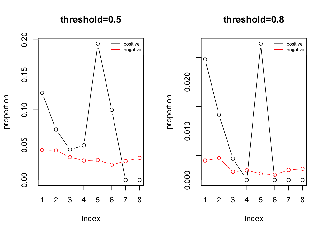

res1 = summary_by_dist(0.5, dist_range = c(0, 1e4, 5e4, 1e5, 3e6))
res2 = summary_by_dist(0.8, dist_range = c(0, 1e4, 5e4, 1e5, 3e6))

par(mfrow = c(1,2))
plot(res1$pos, type = 'b', ylab = 'proportion', ylim = c(0, 0.15),  main = 'threshold=0.5')
points(res1$neg, type = 'b', col = 'red')
legend('topright', legend =  c('positive', 'negative'), col = c('black', 'red'), lty = 1, cex = 0.6)


plot(res2$pos, type = 'b', ylab = 'proportion', ylim = c(0, 0.03), main = 'threshold=0.8')
points(res2$neg, type = 'b', col = 'red')
legend('topright', legend =  c('positive', 'negative'), col = c('black', 'red'), lty = 1, cex = 0.6)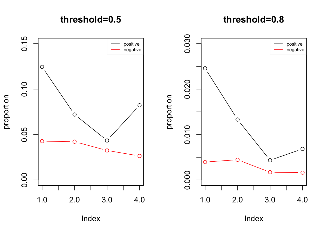

Session information

sessionInfo()

R version 3.6.3 (2020-02-29)
Platform: x86_64-apple-darwin15.6.0 (64-bit)
Running under: macOS Catalina 10.15.5

Matrix products: default
BLAS:   /Library/Frameworks/R.framework/Versions/3.6/Resources/lib/libRblas.0.dylib
LAPACK: /Library/Frameworks/R.framework/Versions/3.6/Resources/lib/libRlapack.dylib

locale:
[1] en_US.UTF-8/en_US.UTF-8/en_US.UTF-8/C/en_US.UTF-8/en_US.UTF-8

attached base packages:
[1] stats     graphics  grDevices utils     datasets  methods   base     

other attached packages:
[1] workflowr_1.6.1

loaded via a namespace (and not attached):
 [1] Rcpp_1.0.4      rprojroot_1.3-2 digest_0.6.25   later_1.0.0    
 [5] R6_2.4.1        backports_1.1.5 git2r_0.26.1    magrittr_1.5   
 [9] evaluate_0.14   highr_0.8       stringi_1.4.6   rlang_0.4.5    
[13] fs_1.3.2        promises_1.1.0  whisker_0.4     rmarkdown_2.1  
[17] tools_3.6.3     stringr_1.4.0   glue_1.3.2      httpuv_1.5.2   
[21] xfun_0.12       yaml_2.2.1      compiler_3.6.3  htmltools_0.4.0
[25] knitr_1.28