model_all_feature
Yunqi Yang
8/18/2020
Last updated: 2020-08-18
Checks: 6 1
Knit directory: gene_level_fine_mapping/
This reproducible R Markdown analysis was created with workflowr (version 1.6.1). The Checks tab describes the reproducibility checks that were applied when the results were created. The Past versions tab lists the development history.
Great! Since the R Markdown file has been committed to the Git repository, you know the exact version of the code that produced these results.
Great job! The global environment was empty. Objects defined in the global environment can affect the analysis in your R Markdown file in unknown ways. For reproduciblity it’s best to always run the code in an empty environment.
The command set.seed(20200622) was run prior to running the code in the R Markdown file. Setting a seed ensures that any results that rely on randomness, e.g. subsampling or permutations, are reproducible.
Great job! Recording the operating system, R version, and package versions is critical for reproducibility.
Nice! There were no cached chunks for this analysis, so you can be confident that you successfully produced the results during this run.
Using absolute paths to the files within your workflowr project makes it difficult for you and others to run your code on a different machine. Change the absolute path(s) below to the suggested relative path(s) to make your code more reproducible.
| absolute | relative |
|---|---|
| /Users/nicholeyang/Desktop/gene_level_fine_mapping/data/train_all.RData | data/train_all.RData |
Great! You are using Git for version control. Tracking code development and connecting the code version to the results is critical for reproducibility.
The results in this page were generated with repository version 6d17ffc. See the Past versions tab to see a history of the changes made to the R Markdown and HTML files.
Note that you need to be careful to ensure that all relevant files for the analysis have been committed to Git prior to generating the results (you can use wflow_publish or wflow_git_commit). workflowr only checks the R Markdown file, but you know if there are other scripts or data files that it depends on. Below is the status of the Git repository when the results were generated:
Ignored files:
    Ignored:    .DS_Store
    Ignored:    .Rhistory
    Ignored:    .Rproj.user/
    Ignored:    analysis/.DS_Store
    Ignored:    analysis/.RData
    Ignored:    analysis/.Rhistory

Untracked files:
    Untracked:  analysis/atac_eqtl.Rmd
    Untracked:  data/hic_eqtl.RData
    Untracked:  data/train_add_hic.RData
    Untracked:  data/train_all.RData

Unstaged changes:
    Modified:   analysis/add_hic_feature.Rmd
Note that any generated files, e.g. HTML, png, CSS, etc., are not included in this status report because it is ok for generated content to have uncommitted changes.
These are the previous versions of the repository in which changes were made to the R Markdown (analysis/fit_all_feature.Rmd) and HTML (docs/fit_all_feature.html) files. If you’ve configured a remote Git repository (see ?wflow_git_remote), click on the hyperlinks in the table below to view the files as they were in that past version.
| File | Version | Author | Date | Message |
|---|---|---|---|---|
| Rmd | 6d17ffc | yunqiyang0215 | 2020-08-18 | wflow_publish(“analysis/fit_all_feature.Rmd”) |
library(ggplot2)
library(dplyr)
Attaching package: 'dplyr'The following objects are masked from 'package:stats':
filter, lagThe following objects are masked from 'package:base':
intersect, setdiff, setequal, unionrequire(PRROC)Loading required package: PRROCload('/Users/nicholeyang/Desktop/gene_level_fine_mapping/data/train_all.RData')
head(train_all_sig) gene_name snp_loc38 variant_id UTR5 UTR3 exon intron
1 A1BG chr19:57866502 chr19_57866502_T_C_b38 0 0 0 0
2 A1BG chr19:58059544 chr19_58059544_T_G_b38 0 0 0 0
3 A1BG chr19:58170494 chr19_58170494_G_T_b38 0 0 0 0
4 A1BG chr19:58228973 chr19_58228973_T_G_b38 0 0 0 0
5 A1BG chr19:58330182 chr19_58330182_C_T_b38 0 0 0 0
6 A1BG chr19:58359927 chr19_58359927_G_A_b38 0 0 0 0
upstream tss_dist_to_snp y Mon Mac0 Mac1 Mac2 Neu MK EP Ery FoeT nCD4 tCD4
1 0 481132 0 0 0 0 0 0 0 0 0 0 0 0
2 0 288090 0 0 0 0 0 0 0 0 0 0 0 0
3 0 177140 0 0 0 0 0 0 0 0 0 0 0 0
4 0 118661 0 0 0 0 0 0 0 0 0 0 0 0
5 0 17452 1 0 0 0 0 0 0 0 0 0 0 0
6 0 6428 1 0 0 0 0 0 0 0 0 0 0 0
aCD4 naCD4 nCD8 tCD8 nB tB correlation
1 0 0 0 0 0 0 0
2 0 0 0 0 0 0 0
3 0 0 0 0 0 0 0
4 0 0 0 0 0 0 0
5 0 0 0 0 0 0 0
6 0 0 0 0 0 0 0process HiC feature
# create unified HiC feature
hic = apply(train_all_sig[, c(11:27)], 1, sum)
train_all_sig$hic = ifelse(hic>0, 1, 0)

# add interaction term based on distance
train_all_sig$hic_dist1 = ifelse(train_all_sig$hic>0 & train_all_sig$tss_dist_to_snp < 5e4, 1, 0)
train_all_sig$hic_dist2 = ifelse(train_all_sig$hic>0 & train_all_sig$tss_dist_to_snp > 5e4 & train_all_sig$tss_dist_to_snp < 1e5, 1, 0)
train_all_sig$hic_dist3 = ifelse(train_all_sig$hic>0 & train_all_sig$tss_dist_to_snp > 1e5, 1, 0)
process ATAC feature
train_all_sig$atac = ifelse(train_all_sig$correlation > 0.5, 1, 0)transform tss_dist_to_snp, use exponential decay: exp(-d/sigma)
sigma = 1e5
train_all_sig$weight = exp(-train_all_sig$tss_dist_to_snp/sigma)
split data and fit models
# split data in the same way
set.seed(1)
n = dim(train_all_sig)[1]
indx = sample(1:n, round(2*n/3), replace = FALSE)
train = train_all_sig[indx, ]
test = train_all_sig[-indx, ]
before adding HiC and ATAC
# fit model and evaluate performance
fit1 = glm(y ~ UTR5 + UTR3 + intron + upstream + exon + weight, data = train, family = "binomial")
summary(fit1)
Call:
glm(formula = y ~ UTR5 + UTR3 + intron + upstream + exon + weight,
    family = "binomial", data = train)

Deviance Residuals:
    Min       1Q   Median       3Q      Max
-2.4294  -0.1205  -0.0617  -0.0513   3.6728

Coefficients:
            Estimate Std. Error z value Pr(>|z|)
(Intercept) -6.74430    0.10582 -63.733  < 2e-16 ***
UTR5         3.18811    0.21524  14.812  < 2e-16 ***
UTR3         1.64574    0.21529   7.644  2.1e-14 ***
intron       3.09218    0.09313  33.203  < 2e-16 ***
upstream     3.22812    0.18851  17.124  < 2e-16 ***
exon         3.64875    0.28856  12.645  < 2e-16 ***
weight       5.99642    0.13693  43.791  < 2e-16 ***
---
Signif. codes:  0 '***' 0.001 '**' 0.01 '*' 0.05 '.' 0.1 ' ' 1

(Dispersion parameter for binomial family taken to be 1)

    Null deviance: 19460.5  on 44304  degrees of freedom
Residual deviance:  7409.4  on 44298  degrees of freedom
AIC: 7423.4

Number of Fisher Scoring iterations: 8
pred.probs=predict(fit1,test,type="response")
glm.pred = rep(0, length(pred.probs))
glm.pred[pred.probs>0.5]= 1
table(glm.pred, test$y)
glm.pred     0     1
       0 20703   488
       1   149   812
fg <- pred.probs[test$y == 1]
bg <- pred.probs[test$y== 0]
# ROC Curve
roc <- roc.curve(scores.class0 = fg, scores.class1 = bg, curve = T)
plot(roc)
# PR Curve
pr <- pr.curve(scores.class0 = fg, scores.class1 = bg, curve = T)
plot(pr)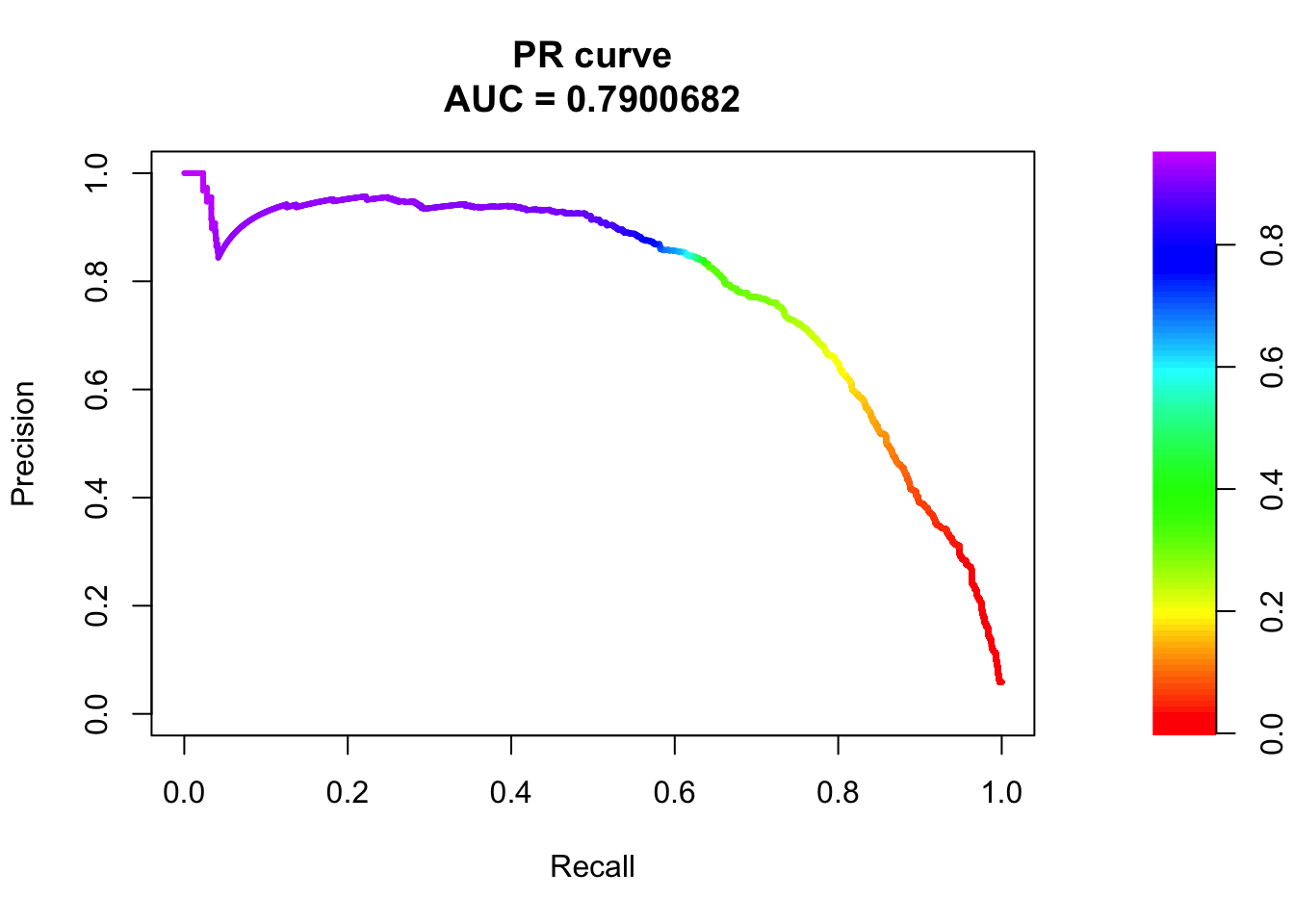
after adding HiC and ATAC
# fit model and evaluate performance
fit2 = glm(y ~ UTR5 + UTR3 + intron + upstream + exon + weight + hic_dist1 + hic_dist2 + hic_dist3 + atac, data = train, family = "binomial")
summary(fit2)
Call:
glm(formula = y ~ UTR5 + UTR3 + intron + upstream + exon + weight +
    hic_dist1 + hic_dist2 + hic_dist3 + atac, family = "binomial",
    data = train)

Deviance Residuals:
    Min       1Q   Median       3Q      Max
-2.4880  -0.1210  -0.0616  -0.0500   3.6922

Coefficients:
            Estimate Std. Error z value Pr(>|z|)
(Intercept) -6.81573    0.11508 -59.226  < 2e-16 ***
UTR5         3.12431    0.21598  14.465  < 2e-16 ***
UTR3         1.68061    0.21592   7.784 7.05e-15 ***
intron       3.08143    0.09334  33.012  < 2e-16 ***
upstream     3.16131    0.18929  16.701  < 2e-16 ***
exon         3.65713    0.28967  12.625  < 2e-16 ***
weight       6.06381    0.14656  41.374  < 2e-16 ***
hic_dist1   -0.23850    0.12405  -1.923   0.0545 .
hic_dist2    0.32256    0.19664   1.640   0.1009
hic_dist3    0.18278    0.26650   0.686   0.4928
atac         0.56209    0.13369   4.204 2.62e-05 ***
---
Signif. codes:  0 '***' 0.001 '**' 0.01 '*' 0.05 '.' 0.1 ' ' 1

(Dispersion parameter for binomial family taken to be 1)

    Null deviance: 19460.5  on 44304  degrees of freedom
Residual deviance:  7385.5  on 44294  degrees of freedom
AIC: 7407.5

Number of Fisher Scoring iterations: 8
pred.probs=predict(fit2,test,type="response")
glm.pred = rep(0, length(pred.probs))
glm.pred[pred.probs>0.5]= 1
table(glm.pred, test$y)
glm.pred     0     1
       0 20704   489
       1   148   811
fg <- pred.probs[test$y == 1]
bg <- pred.probs[test$y== 0]
# ROC Curve
roc <- roc.curve(scores.class0 = fg, scores.class1 = bg, curve = T)
plot(roc)
# PR Curve
pr <- pr.curve(scores.class0 = fg, scores.class1 = bg, curve = T)
plot(pr)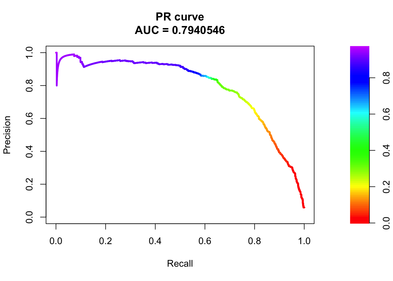
# fit model and evaluate performance
fit3 = glm(y ~ UTR5 + UTR3 + intron + upstream + exon + weight + hic + atac, data = train, family = "binomial")
summary(fit3)
Call:
glm(formula = y ~ UTR5 + UTR3 + intron + upstream + exon + weight +
    hic + atac, family = "binomial", data = train)

Deviance Residuals:
    Min       1Q   Median       3Q      Max
-2.4828  -0.1200  -0.0623  -0.0513   3.6727

Coefficients:
            Estimate Std. Error z value Pr(>|z|)
(Intercept) -6.74369    0.10778 -62.570  < 2e-16 ***
UTR5         3.14405    0.21569  14.577  < 2e-16 ***
UTR3         1.67370    0.21541   7.770 7.85e-15 ***
intron       3.07916    0.09329  33.006  < 2e-16 ***
upstream     3.17839    0.18906  16.811  < 2e-16 ***
exon         3.65627    0.28894  12.654  < 2e-16 ***
weight       5.96852    0.13729  43.475  < 2e-16 ***
hic         -0.07324    0.10195  -0.718    0.473
atac         0.56601    0.13373   4.233 2.31e-05 ***
---
Signif. codes:  0 '***' 0.001 '**' 0.01 '*' 0.05 '.' 0.1 ' ' 1

(Dispersion parameter for binomial family taken to be 1)

    Null deviance: 19460.5  on 44304  degrees of freedom
Residual deviance:  7391.8  on 44296  degrees of freedom
AIC: 7409.8

Number of Fisher Scoring iterations: 8
pred.probs=predict(fit3,test,type="response")
glm.pred = rep(0, length(pred.probs))
glm.pred[pred.probs>0.5]= 1
table(glm.pred, test$y)
glm.pred     0     1
       0 20701   489
       1   151   811
fg <- pred.probs[test$y == 1]
bg <- pred.probs[test$y== 0]
# ROC Curve
roc <- roc.curve(scores.class0 = fg, scores.class1 = bg, curve = T)
plot(roc)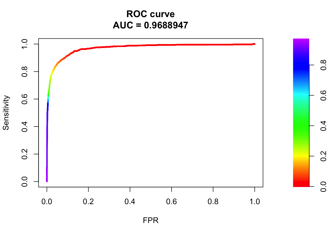
# PR Curve
pr <- pr.curve(scores.class0 = fg, scores.class1 = bg, curve = T)
plot(pr)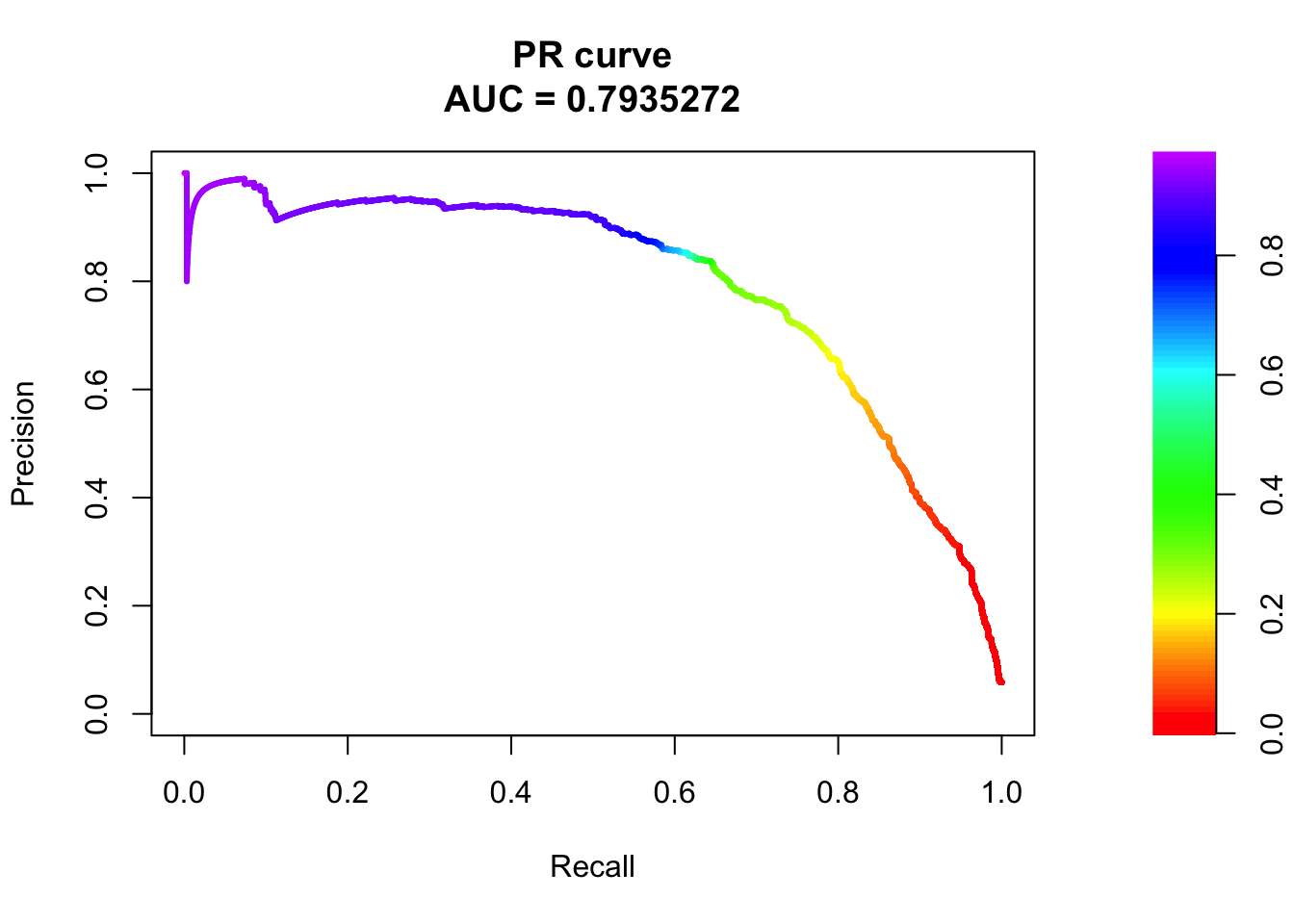
# fit model and evaluate performance
fit4 = glm(y ~ UTR5 + UTR3 + intron + upstream + exon + weight*hic + atac, data = train, family = "binomial")
summary(fit4)
Call:
glm(formula = y ~ UTR5 + UTR3 + intron + upstream + exon + weight *
    hic + atac, family = "binomial", data = train)

Deviance Residuals:
    Min       1Q   Median       3Q      Max
-2.4907  -0.1220  -0.0637  -0.0496   3.6960

Coefficients:
            Estimate Std. Error z value Pr(>|z|)
(Intercept) -6.82962    0.11678 -58.485  < 2e-16 ***
UTR5         3.12113    0.21602  14.449  < 2e-16 ***
UTR3         1.67787    0.21577   7.776 7.47e-15 ***
intron       3.08069    0.09335  33.001  < 2e-16 ***
upstream     3.16095    0.18949  16.682  < 2e-16 ***
exon         3.65877    0.28976  12.627  < 2e-16 ***
weight       6.08206    0.14868  40.908  < 2e-16 ***
hic          0.52205    0.27600   1.891   0.0586 .
atac         0.56422    0.13359   4.224 2.40e-05 ***
weight:hic  -0.87175    0.38400  -2.270   0.0232 *
---
Signif. codes:  0 '***' 0.001 '**' 0.01 '*' 0.05 '.' 0.1 ' ' 1

(Dispersion parameter for binomial family taken to be 1)

    Null deviance: 19460.5  on 44304  degrees of freedom
Residual deviance:  7386.9  on 44295  degrees of freedom
AIC: 7406.9

Number of Fisher Scoring iterations: 8
pred.probs=predict(fit4,test,type="response")
glm.pred = rep(0, length(pred.probs))
glm.pred[pred.probs>0.5]= 1
table(glm.pred, test$y)
glm.pred     0     1
       0 20702   489
       1   150   811
fg <- pred.probs[test$y == 1]
bg <- pred.probs[test$y== 0]
# ROC Curve
roc <- roc.curve(scores.class0 = fg, scores.class1 = bg, curve = T)
plot(roc)
# PR Curve
pr <- pr.curve(scores.class0 = fg, scores.class1 = bg, curve = T)
plot(pr)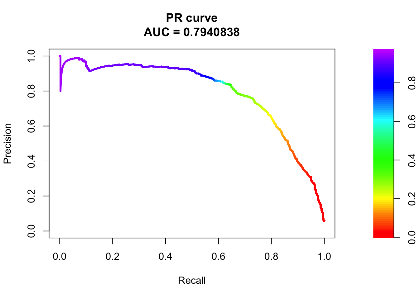
sessionInfo()R version 3.6.3 (2020-02-29)
Platform: x86_64-apple-darwin15.6.0 (64-bit)
Running under: macOS Catalina 10.15.5
Matrix products: default
BLAS: /Library/Frameworks/R.framework/Versions/3.6/Resources/lib/libRblas.0.dylib
LAPACK: /Library/Frameworks/R.framework/Versions/3.6/Resources/lib/libRlapack.dylib
locale:
[1] en_US.UTF-8/en_US.UTF-8/en_US.UTF-8/C/en_US.UTF-8/en_US.UTF-8
attached base packages:
[1] stats graphics grDevices utils datasets methods base
other attached packages:
[1] PRROC_1.3.1 dplyr_0.8.5 ggplot2_3.3.0 workflowr_1.6.1
loaded via a namespace (and not attached):
[1] Rcpp_1.0.4 compiler_3.6.3 pillar_1.4.3 later_1.0.0
[5] git2r_0.26.1 highr_0.8 tools_3.6.3 digest_0.6.25
[9] evaluate_0.14 lifecycle_0.2.0 tibble_3.0.1 gtable_0.3.0
[13] pkgconfig_2.0.3 rlang_0.4.5 rstudioapi_0.11 yaml_2.2.1
[17] xfun_0.12 withr_2.1.2 stringr_1.4.0 knitr_1.28
[21] fs_1.3.2 vctrs_0.2.4 rprojroot_1.3-2 grid_3.6.3
[25] tidyselect_1.0.0 glue_1.3.2 R6_2.4.1 rmarkdown_2.1
[29] purrr_0.3.3 magrittr_1.5 whisker_0.4 backports_1.1.5
[33] scales_1.1.0 promises_1.1.0 htmltools_0.4.0 ellipsis_0.3.0
[37] assertthat_0.2.1 colorspace_1.4-1 httpuv_1.5.2 stringi_1.4.6
[41] munsell_0.5.0 crayon_1.3.4