distance function

Last updated: 2020-07-30

Checks: 6 1

Knit directory: gene_level_fine_mapping/

This reproducible R Markdown analysis was created with workflowr (version 1.6.1). The Checks tab describes the reproducibility checks that were applied when the results were created. The Past versions tab lists the development history.

R Markdown file: up-to-date

Great! Since the R Markdown file has been committed to the Git repository, you know the exact version of the code that produced these results.

Environment: empty

Great job! The global environment was empty. Objects defined in the global environment can affect the analysis in your R Markdown file in unknown ways. For reproduciblity it’s best to always run the code in an empty environment.

Seed: set.seed(20200622)

The command set.seed(20200622) was run prior to running the code in the R Markdown file. Setting a seed ensures that any results that rely on randomness, e.g. subsampling or permutations, are reproducible.

Session information: recorded

Great job! Recording the operating system, R version, and package versions is critical for reproducibility.

Cache: none

Nice! There were no cached chunks for this analysis, so you can be confident that you successfully produced the results during this run.

File paths: absolute

Using absolute paths to the files within your workflowr project makes it difficult for you and others to run your code on a different machine. Change the absolute path(s) below to the suggested relative path(s) to make your code more reproducible.

absolute	relative
/Users/nicholeyang/Desktop/gene_level_fine_mapping/data/training.RData	data/training.RData

Repository version: fceec56

Great! You are using Git for version control. Tracking code development and connecting the code version to the results is critical for reproducibility.

The results in this page were generated with repository version fceec56. See the Past versions tab to see a history of the changes made to the R Markdown and HTML files.

Note that you need to be careful to ensure that all relevant files for the analysis have been committed to Git prior to generating the results (you can use wflow_publish or wflow_git_commit). workflowr only checks the R Markdown file, but you know if there are other scripts or data files that it depends on. Below is the status of the Git repository when the results were generated:


Ignored files:
    Ignored:    .DS_Store
    Ignored:    .Rhistory
    Ignored:    .Rproj.user/

Note that any generated files, e.g. HTML, png, CSS, etc., are not included in this status report because it is ok for generated content to have uncommitted changes.

These are the previous versions of the repository in which changes were made to the R Markdown (analysis/dist_functions.Rmd) and HTML (docs/dist_functions.html) files. If you’ve configured a remote Git repository (see ?wflow_git_remote), click on the hyperlinks in the table below to view the files as they were in that past version.

File	Version	Author	Date	Message
Rmd	fceec56	yunqiyang0215	2020-07-30	wflow_publish(“analysis/dist_functions.Rmd”)

Comment:

Tried exponential decay function and gaussian decay function with 4 different sigma values. I think sigma values and which decay function to use don’t have large impact on the ROC and PR curve.
However, the coefficient for ‘weight’ variable changes a lot when vary sigma values. We might want to use a sigma value based on the shape of the decay curve, which one looks more reasonable in terms of biology.

library(ggplot2)
library(dplyr)


Attaching package: 'dplyr'

The following objects are masked from 'package:stats':

    filter, lag

The following objects are masked from 'package:base':

    intersect, setdiff, setequal, union

require(PRROC)

Loading required package: PRROC

load("/Users/nicholeyang/Desktop/gene_level_fine_mapping/data/training.RData")

## remove NAs
dat = rbind(train_pos_all, train_neg_all)
NAs = apply(dat, 1, function(x) sum(is.na(x)))
dat = dat[NAs == 0, ]

data overview

head(dat)

  gene_name             variant_id UTR5 UTR3 exon intron upstream
1    LRRC39 chr1_100178174_A_G_b38    1    0    0      0        0
2     EXTL2 chr1_100895622_C_T_b38    0    0    0      0        1
3     KIF1B  chr1_10211630_C_G_b38    1    0    0      0        0
6  SLC25A24 chr1_108199501_C_G_b38    0    0    0      1        0
8     TAF13 chr1_109076695_G_A_b38    0    0    0      0        1
9  C1orf194 chr1_109113015_C_A_b38    0    0    0      1        0
  tss_dist_to_snp y
1              41 1
2             376 1
3              14 1
6             857 1
8             693 1
9             268 1

# number of observations in the dataset 
dim(dat)[1]

[1] 65858

sum(dat$y == 1)  # positive pairs

[1] 3828

sum(dat$y == 0)  # negative pairs

[1] 62030

proportion of features

par(mfrow = c(1,2))

# proportion of features in the positive set
tot_count = apply(dat[dat$y==1, c(3:7)], 2, function(x) sum(x == 1))
barplot(tot_count/dim(dat[dat$y==1, ])[1], las = 2, main = 'feature proportion in positive set')

# proportion of features in the negative set
tot_count = apply(dat[dat$y==0, c(3:7)], 2, function(x) sum(x == 1))
barplot(tot_count/dim(dat[dat$y==0, ])[1], ylim = c(0, 0.01), las = 2, main = 'feature proportion in negative set')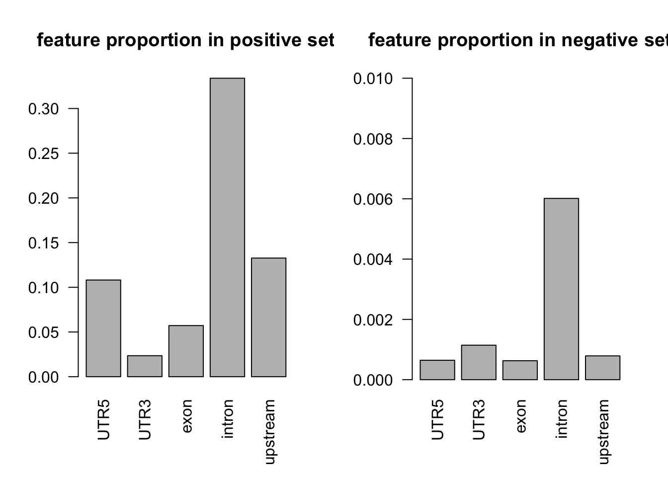

play around tss feature

summary(dat$tss_dist_to_snp)

   Min. 1st Qu.  Median    Mean 3rd Qu.    Max. 
      0   91718  221543  232448  364130 2176373

summary(dat[dat$y==1, ]$tss_dist_to_snp)  # dist_to_tss in positive set

    Min.  1st Qu.   Median     Mean  3rd Qu.     Max. 
     0.0    297.8   3009.5  20349.3  17583.0 946399.0

summary(dat[dat$y==0, ]$tss_dist_to_snp)  # dist_to_tss in negative set

   Min. 1st Qu.  Median    Mean 3rd Qu.    Max. 
      0  112052  237240  245537  372089 2176373

two decay functions: exponential decay and gaussian decay.

the decay functions look like under the distance range we have.

gaussian_decay = function(sigma, d){
  k = exp(-d^2/sigma^2/2)
  return(k)
}
  
exp_decay = function(sigma, d){
  k = exp(-d/sigma)
  return(k)
}

dist = seq(0, 2e7, by = 1e3)
sigmas = c(1e4, 1e5, 1e6, 1e7)

par(mfrow = c(2,2))
plot(gaussian_decay(sigmas[1], dist), type = 'l', ylab = 'weight', xlab = 'distance')
plot(gaussian_decay(sigmas[2], dist), type = 'l', ylab = 'weight', xlab = 'distance')
plot(gaussian_decay(sigmas[3], dist), type = 'l', ylab = 'weight', xlab = 'distance')
plot(gaussian_decay(sigmas[4], dist), type = 'l', ylab = 'weight', xlab = 'distance')

par(mfrow = c(2,2))
plot(exp_decay(sigmas[1], dist), type = 'l', ylab = 'weight', xlab = 'distance')
plot(exp_decay(sigmas[2], dist), type = 'l', ylab = 'weight', xlab = 'distance')
plot(exp_decay(sigmas[3], dist), type = 'l', ylab = 'weight', xlab = 'distance')
plot(exp_decay(sigmas[4], dist), type = 'l', ylab = 'weight', xlab = 'distance')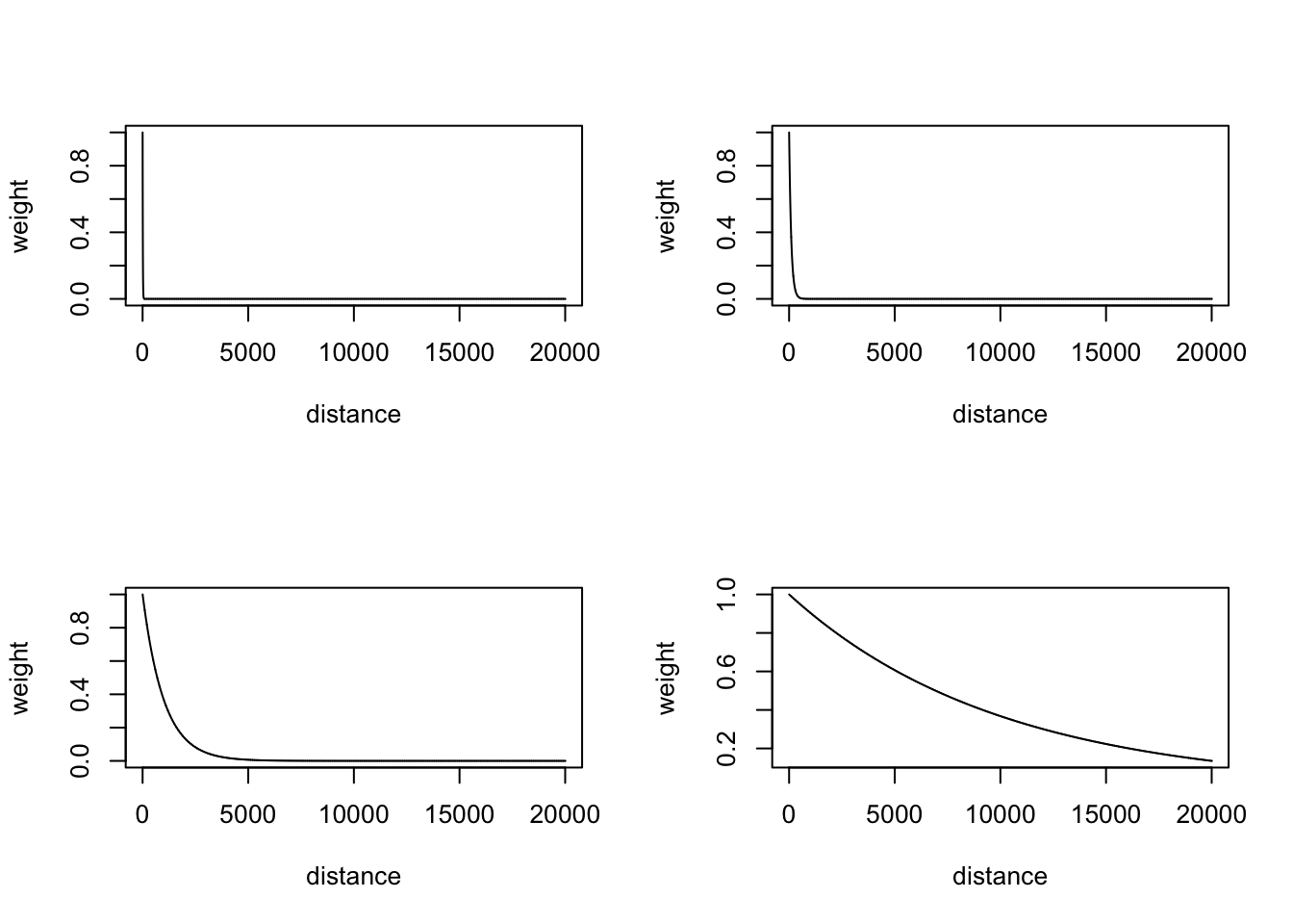

exponential decay: exp(-d/sigma)

weights = matrix(NA, ncol = length(sigmas), nrow = dim(dat)[1])

for (i in 1:length(sigmas)){
  weights[, i] = exp(-dat$tss_dist_to_snp/sigmas[i])
}

weights = data.frame(weights)
colnames(weights) = c('sig1', 'sig2', 'sig3', 'sig4')


dat2 = cbind(dat, weights)

ggplot(dat2, aes(x = sig1)) +
  geom_histogram(aes(color = as.factor(y), fill = as.factor(y)), 
                position = "identity", bins = 50, alpha = 0.4) +
  scale_color_manual(values = c("#00AFBB", "#E7B800")) +
  scale_fill_manual(values = c("#00AFBB", "#E7B800"))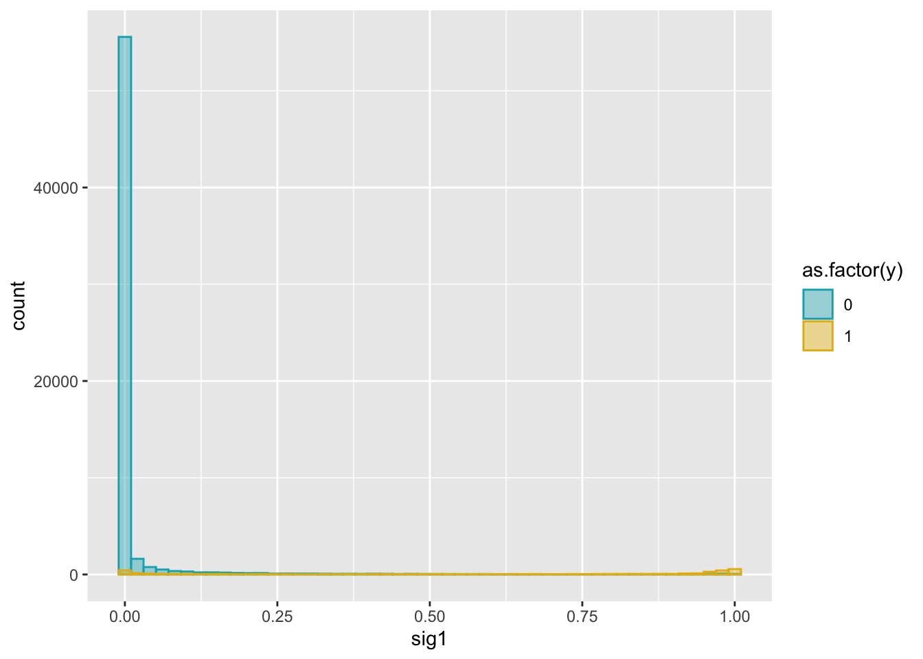

ggplot(dat2, aes(x = sig2)) +
  geom_histogram(aes(color = as.factor(y), fill = as.factor(y)), 
                position = "identity", bins = 50, alpha = 0.4) +
  scale_color_manual(values = c("#00AFBB", "#E7B800")) +
  scale_fill_manual(values = c("#00AFBB", "#E7B800"))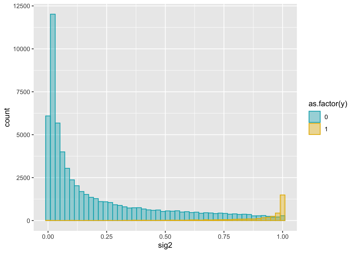

ggplot(dat2, aes(x = sig3)) +
  geom_histogram(aes(color = as.factor(y), fill = as.factor(y)), 
                position = "identity", bins = 50, alpha = 0.4) +
  scale_color_manual(values = c("#00AFBB", "#E7B800")) +
  scale_fill_manual(values = c("#00AFBB", "#E7B800"))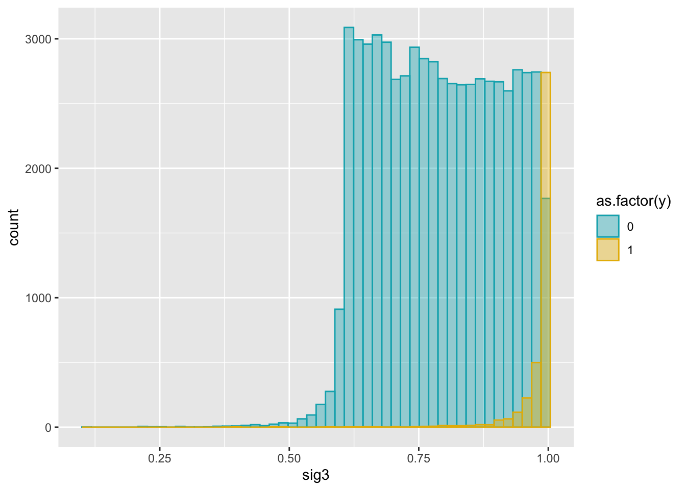

ggplot(dat2, aes(x = sig4)) +
  geom_histogram(aes(color = as.factor(y), fill = as.factor(y)), 
                position = "identity", bins = 50, alpha = 0.4) +
  scale_color_manual(values = c("#00AFBB", "#E7B800")) +
  scale_fill_manual(values = c("#00AFBB", "#E7B800"))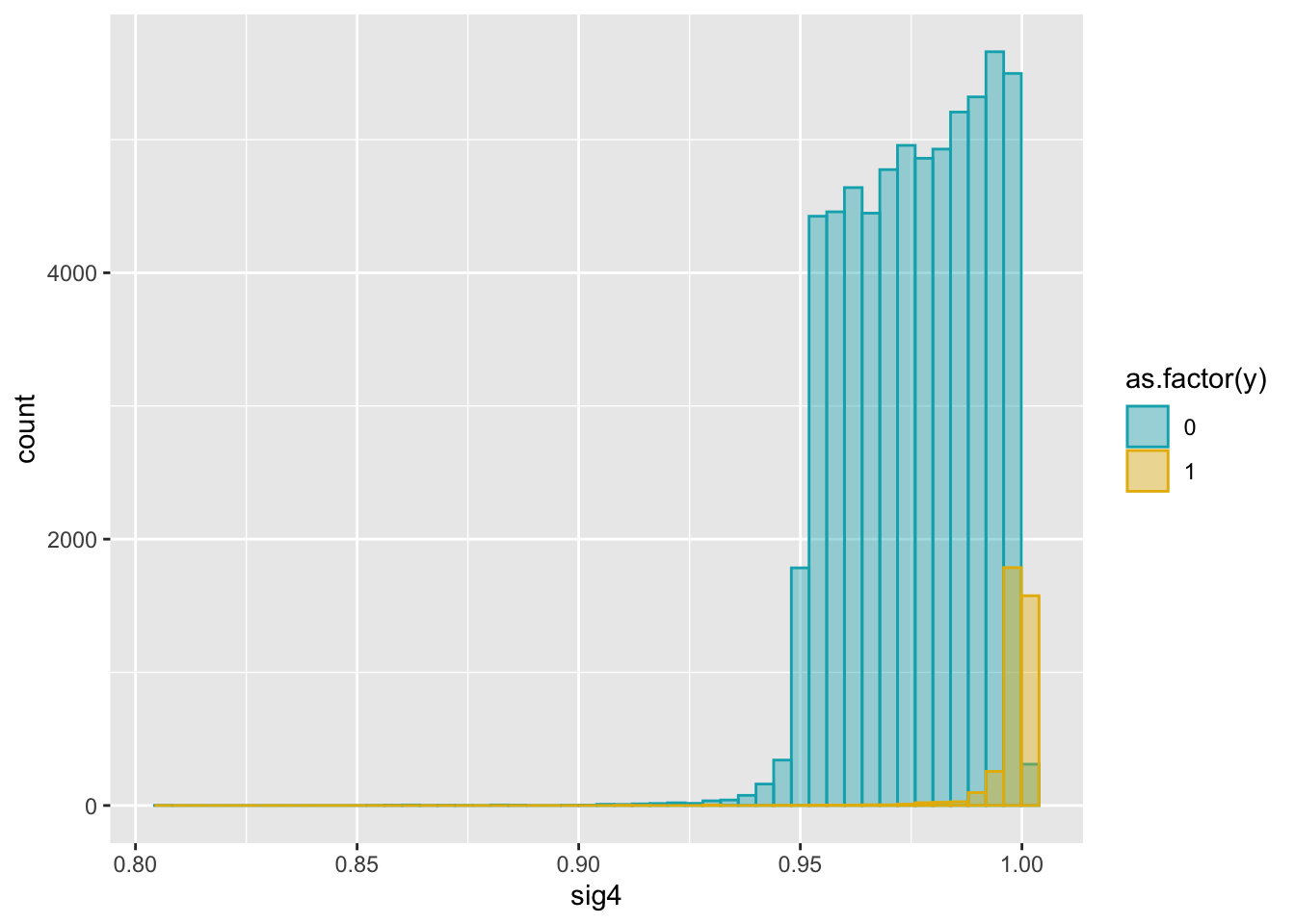

add weight to all feature logsitic regression and plot ROC/PR-AUC

# split data in the same way
set.seed(1)
n = dim(dat2)[1]
indx = sample(1:n, round(2*n/3), replace = FALSE)
train = dat2[indx, ]
test = dat2[-indx, ]

# fit model and evaluate performance
fit.sig1 = glm(y ~ UTR5 + UTR3 + intron + upstream + exon + sig1, data = train, family = "binomial")
fit.sig2 = glm(y ~ UTR5 + UTR3 + intron + upstream + exon + sig2, data = train, family = "binomial")
fit.sig3 = glm(y ~ UTR5 + UTR3 + intron + upstream + exon + sig3, data = train, family = "binomial")
fit.sig4 = glm(y ~ UTR5 + UTR3 + intron + upstream + exon + sig4, data = train, family = "binomial")

Warning: glm.fit: fitted probabilities numerically 0 or 1 occurred

summary(fit.sig1)


Call:
glm(formula = y ~ UTR5 + UTR3 + intron + upstream + exon + sig1, 
    family = "binomial", data = train)

Deviance Residuals: 
    Min       1Q   Median       3Q      Max  
-2.9152  -0.1623  -0.1623  -0.1623   2.9449  

Coefficients:
            Estimate Std. Error z value Pr(>|z|)    
(Intercept) -4.32317    0.04186 -103.28   <2e-16 ***
UTR5         2.47653    0.24711   10.02   <2e-16 ***
UTR3         2.62234    0.24087   10.89   <2e-16 ***
intron       3.80564    0.09426   40.37   <2e-16 ***
upstream     3.07391    0.23407   13.13   <2e-16 ***
exon         3.86273    0.28180   13.71   <2e-16 ***
sig1         4.75517    0.10058   47.27   <2e-16 ***
---
Signif. codes:  0 '***' 0.001 '**' 0.01 '*' 0.05 '.' 0.1 ' ' 1

(Dispersion parameter for binomial family taken to be 1)

    Null deviance: 19491.1  on 43904  degrees of freedom
Residual deviance:  8353.9  on 43898  degrees of freedom
AIC: 8367.9

Number of Fisher Scoring iterations: 7

summary(fit.sig2)


Call:
glm(formula = y ~ UTR5 + UTR3 + intron + upstream + exon + sig2, 
    family = "binomial", data = train)

Deviance Residuals: 
    Min       1Q   Median       3Q      Max  
-2.3112  -0.1202  -0.0614  -0.0513   3.6728  

Coefficients:
            Estimate Std. Error z value Pr(>|z|)    
(Intercept) -6.74427    0.10647 -63.343  < 2e-16 ***
UTR5         3.29539    0.22171  14.863  < 2e-16 ***
UTR3         1.73510    0.21358   8.124 4.51e-16 ***
intron       2.99398    0.09153  32.710  < 2e-16 ***
upstream     3.38742    0.19178  17.663  < 2e-16 ***
exon         3.42179    0.26956  12.694  < 2e-16 ***
sig2         5.97896    0.13754  43.471  < 2e-16 ***
---
Signif. codes:  0 '***' 0.001 '**' 0.01 '*' 0.05 '.' 0.1 ' ' 1

(Dispersion parameter for binomial family taken to be 1)

    Null deviance: 19491.1  on 43904  degrees of freedom
Residual deviance:  7377.4  on 43898  degrees of freedom
AIC: 7391.4

Number of Fisher Scoring iterations: 8

summary(fit.sig3)


Call:
glm(formula = y ~ UTR5 + UTR3 + intron + upstream + exon + sig3, 
    family = "binomial", data = train)

Deviance Residuals: 
    Min       1Q   Median       3Q      Max  
-2.2665  -0.1581  -0.0356  -0.0088   5.8936  

Coefficients:
            Estimate Std. Error z value Pr(>|z|)    
(Intercept) -28.0741     0.8222 -34.145   <2e-16 ***
UTR5          3.8661     0.2198  17.593   <2e-16 ***
UTR3          1.9822     0.2067   9.589   <2e-16 ***
intron        3.1635     0.0872  36.277   <2e-16 ***
upstream      3.8390     0.1861  20.626   <2e-16 ***
exon          3.7276     0.2574  14.483   <2e-16 ***
sig3         26.6986     0.8565  31.174   <2e-16 ***
---
Signif. codes:  0 '***' 0.001 '**' 0.01 '*' 0.05 '.' 0.1 ' ' 1

(Dispersion parameter for binomial family taken to be 1)

    Null deviance: 19491.1  on 43904  degrees of freedom
Residual deviance:  7740.2  on 43898  degrees of freedom
AIC: 7754.2

Number of Fisher Scoring iterations: 9

summary(fit.sig4)


Call:
glm(formula = y ~ UTR5 + UTR3 + intron + upstream + exon + sig4, 
    family = "binomial", data = train)

Deviance Residuals: 
    Min       1Q   Median       3Q      Max  
-2.2646  -0.1668  -0.0350  -0.0066   6.6521  

Coefficients:
             Estimate Std. Error z value Pr(>|z|)    
(Intercept) -238.0692     7.8574 -30.299   <2e-16 ***
UTR5           3.9500     0.2194  18.004   <2e-16 ***
UTR3           2.0321     0.2061   9.862   <2e-16 ***
intron         3.2035     0.0868  36.905   <2e-16 ***
upstream       3.9113     0.1856  21.077   <2e-16 ***
exon           3.7823     0.2558  14.785   <2e-16 ***
sig4         236.6048     7.8921  29.980   <2e-16 ***
---
Signif. codes:  0 '***' 0.001 '**' 0.01 '*' 0.05 '.' 0.1 ' ' 1

(Dispersion parameter for binomial family taken to be 1)

    Null deviance: 19491.1  on 43904  degrees of freedom
Residual deviance:  7831.3  on 43898  degrees of freedom
AIC: 7845.3

Number of Fisher Scoring iterations: 9

## sigma1
pred.probs=predict(fit.sig1,test,type="response")
glm.pred = rep(0, length(pred.probs))
glm.pred[pred.probs>0.5]= 1
table(glm.pred, test$y)

        
glm.pred     0     1
       0 20527   536
       1   153   737

fg <- pred.probs[test$y == 1]
bg <- pred.probs[test$y== 0]

# ROC Curve    
roc <- roc.curve(scores.class0 = fg, scores.class1 = bg, curve = T)
plot(roc)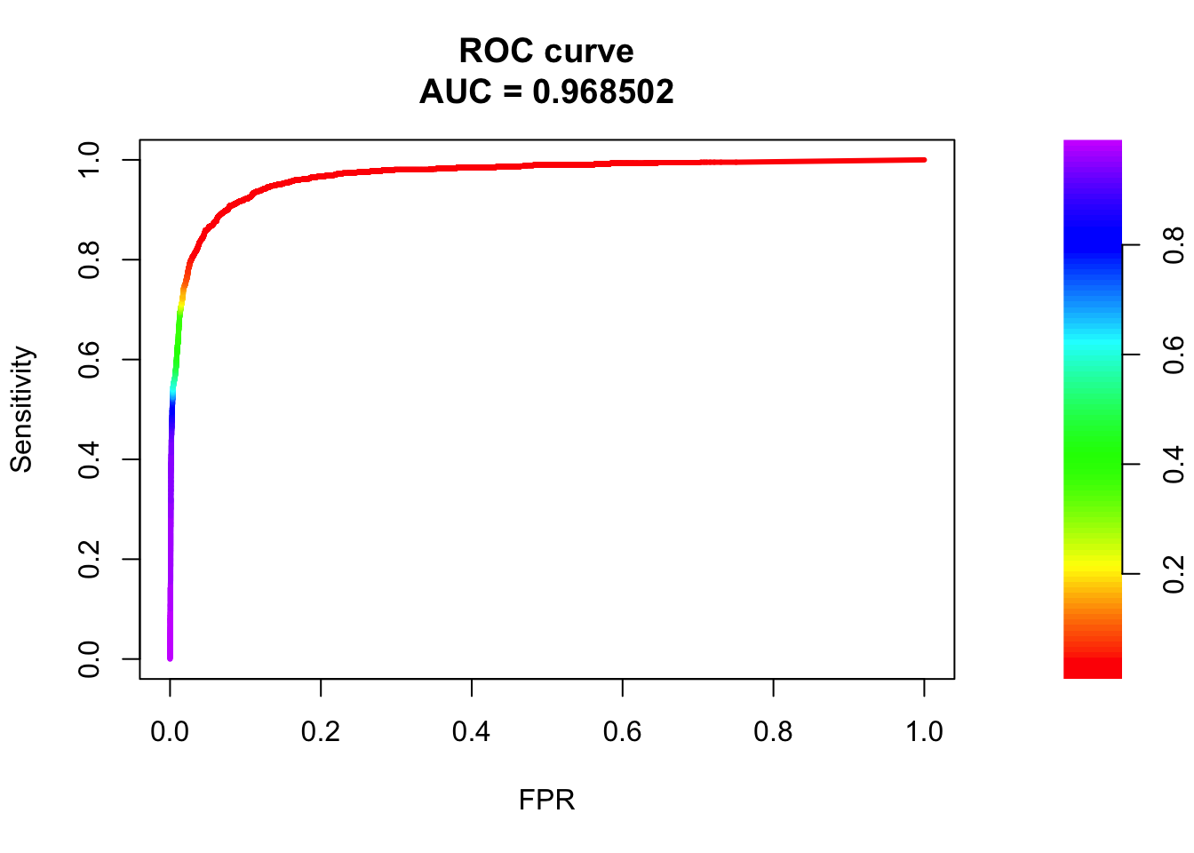

# PR Curve
pr <- pr.curve(scores.class0 = fg, scores.class1 = bg, curve = T)
plot(pr)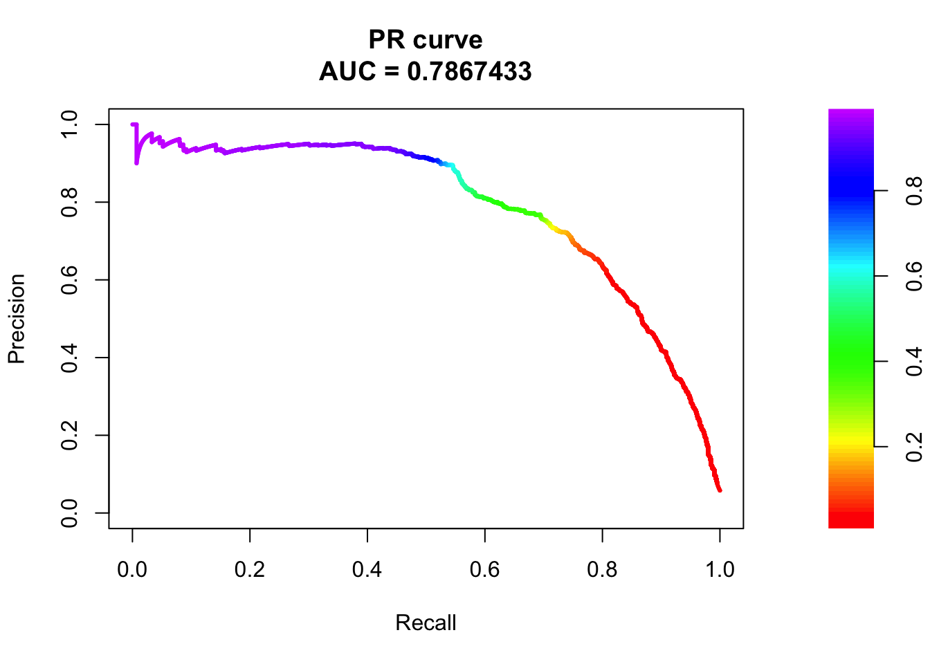

## sigma2
pred.probs=predict(fit.sig2,test,type="response")
glm.pred = rep(0, length(pred.probs))
glm.pred[pred.probs>0.5]= 1
table(glm.pred, test$y)

        
glm.pred     0     1
       0 20539   503
       1   141   770

fg <- pred.probs[test$y == 1]
bg <- pred.probs[test$y== 0]

# ROC Curve    
roc <- roc.curve(scores.class0 = fg, scores.class1 = bg, curve = T)
plot(roc)

# PR Curve
pr <- pr.curve(scores.class0 = fg, scores.class1 = bg, curve = T)
plot(pr)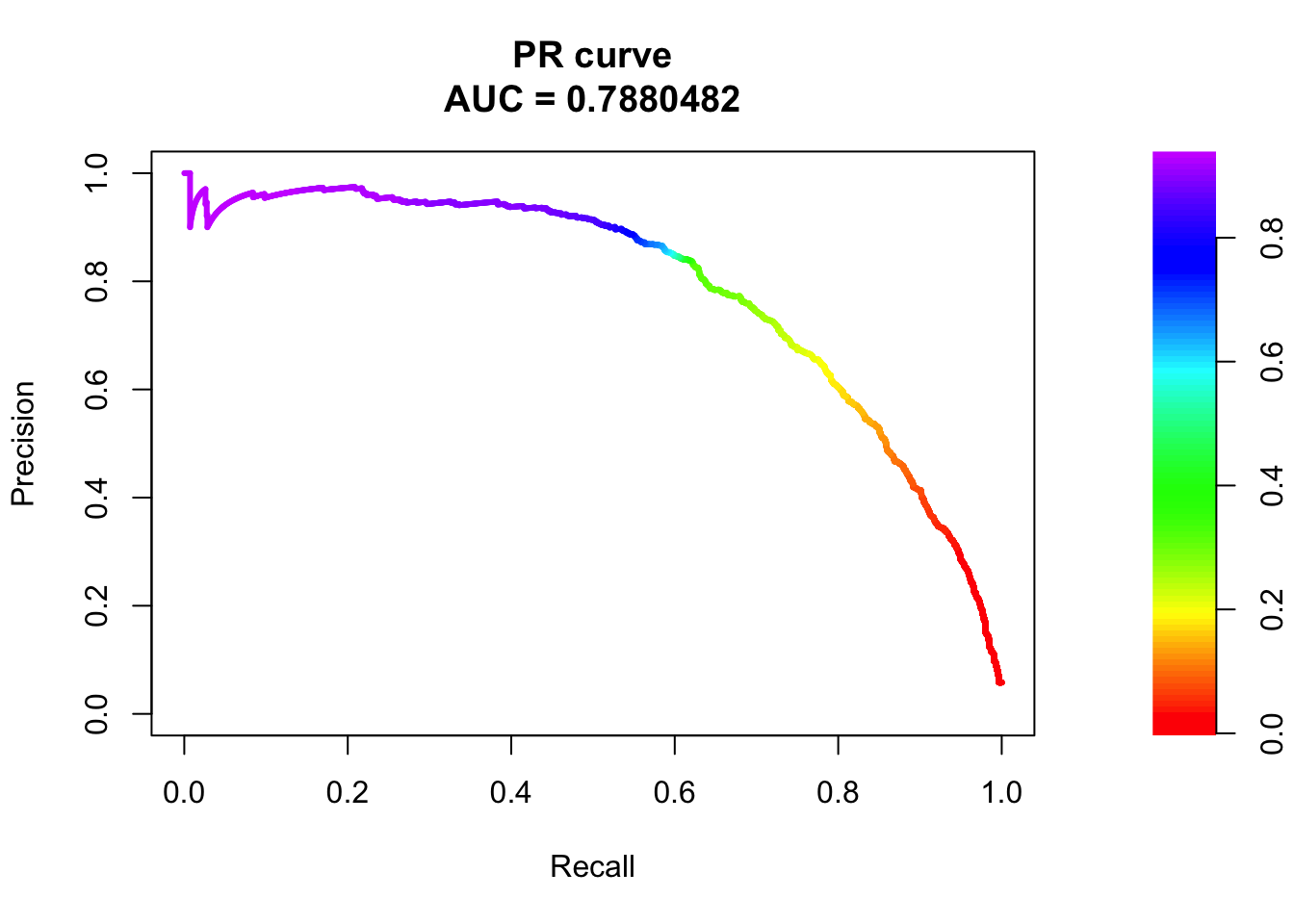

## sigma3
pred.probs=predict(fit.sig3,test,type="response")
glm.pred = rep(0, length(pred.probs))
glm.pred[pred.probs>0.5]= 1
table(glm.pred, test$y)

        
glm.pred     0     1
       0 20524   486
       1   156   787

fg <- pred.probs[test$y == 1]
bg <- pred.probs[test$y== 0]

# ROC Curve    
roc <- roc.curve(scores.class0 = fg, scores.class1 = bg, curve = T)
plot(roc)

# PR Curve
pr <- pr.curve(scores.class0 = fg, scores.class1 = bg, curve = T)
plot(pr)

## sigma4
pred.probs=predict(fit.sig4,test,type="response")
glm.pred = rep(0, length(pred.probs))
glm.pred[pred.probs>0.5]= 1
table(glm.pred, test$y)

        
glm.pred     0     1
       0 20522   479
       1   158   794

fg <- pred.probs[test$y == 1]
bg <- pred.probs[test$y== 0]

# ROC Curve    
roc <- roc.curve(scores.class0 = fg, scores.class1 = bg, curve = T)
plot(roc)

# PR Curve
pr <- pr.curve(scores.class0 = fg, scores.class1 = bg, curve = T)
plot(pr)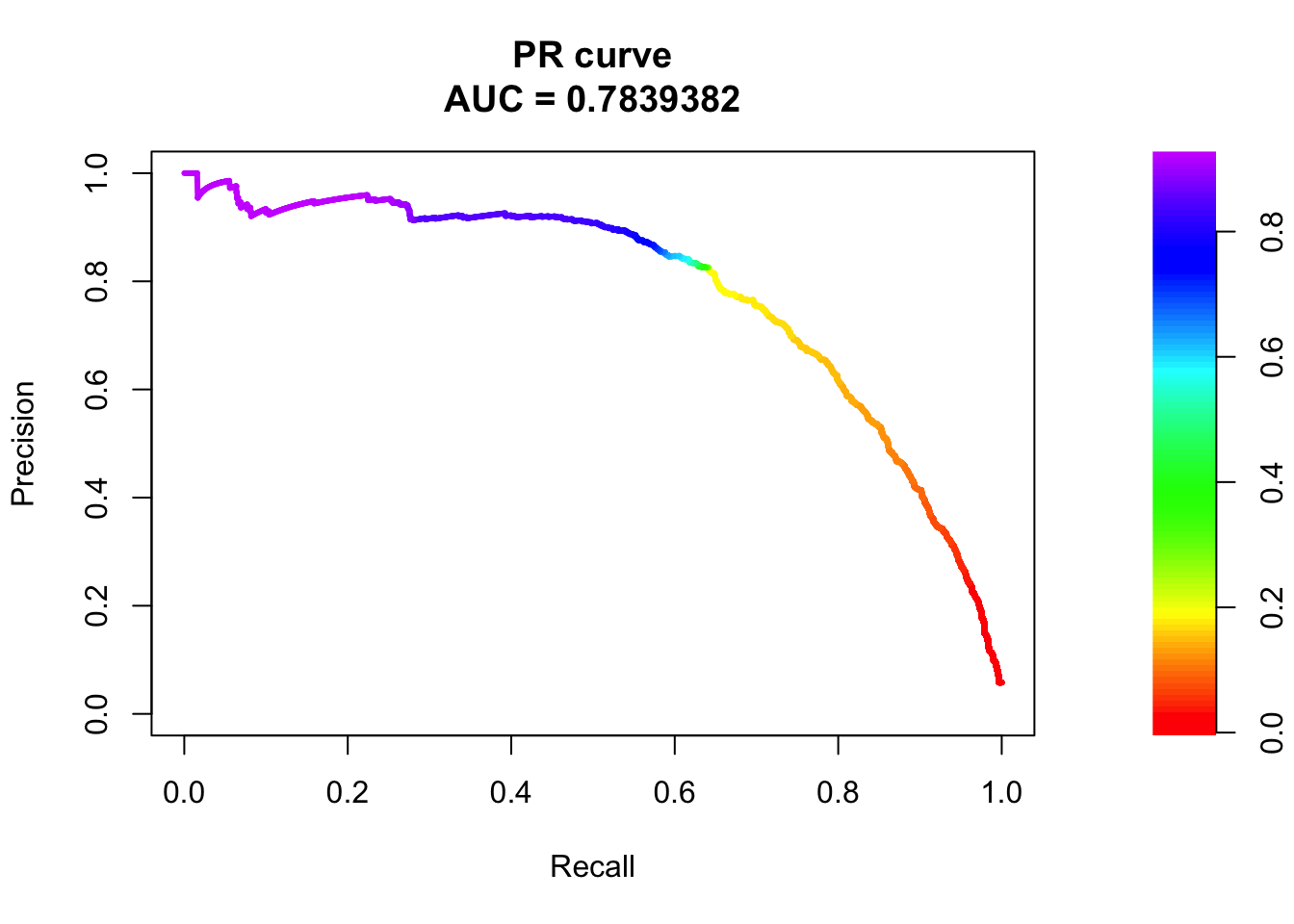

change to gaussian decay function: \(exp(-d^2/2l^2)\)

weights = matrix(NA, ncol = length(sigmas), nrow = dim(dat)[1])

for (i in 1:length(sigmas)){
  weights[, i] = exp(-dat$tss_dist_to_snp^2/sigmas[i]^2)
}

weights = data.frame(weights)
colnames(weights) = c('sig1', 'sig2', 'sig3', 'sig4')

dat2 = cbind(dat, weights)

ggplot(dat2, aes(x = sig1)) +
  geom_histogram(aes(color = as.factor(y), fill = as.factor(y)), 
                position = "identity", bins = 50, alpha = 0.4) +
  scale_color_manual(values = c("#00AFBB", "#E7B800")) +
  scale_fill_manual(values = c("#00AFBB", "#E7B800"))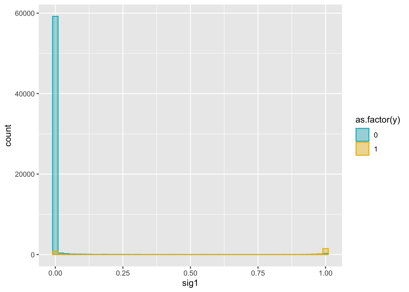

ggplot(dat2, aes(x = sig2)) +
  geom_histogram(aes(color = as.factor(y), fill = as.factor(y)), 
                position = "identity", bins = 50, alpha = 0.4) +
  scale_color_manual(values = c("#00AFBB", "#E7B800")) +
  scale_fill_manual(values = c("#00AFBB", "#E7B800"))

ggplot(dat2, aes(x = sig3)) +
  geom_histogram(aes(color = as.factor(y), fill = as.factor(y)), 
                position = "identity", bins = 50, alpha = 0.4) +
  scale_color_manual(values = c("#00AFBB", "#E7B800")) +
  scale_fill_manual(values = c("#00AFBB", "#E7B800"))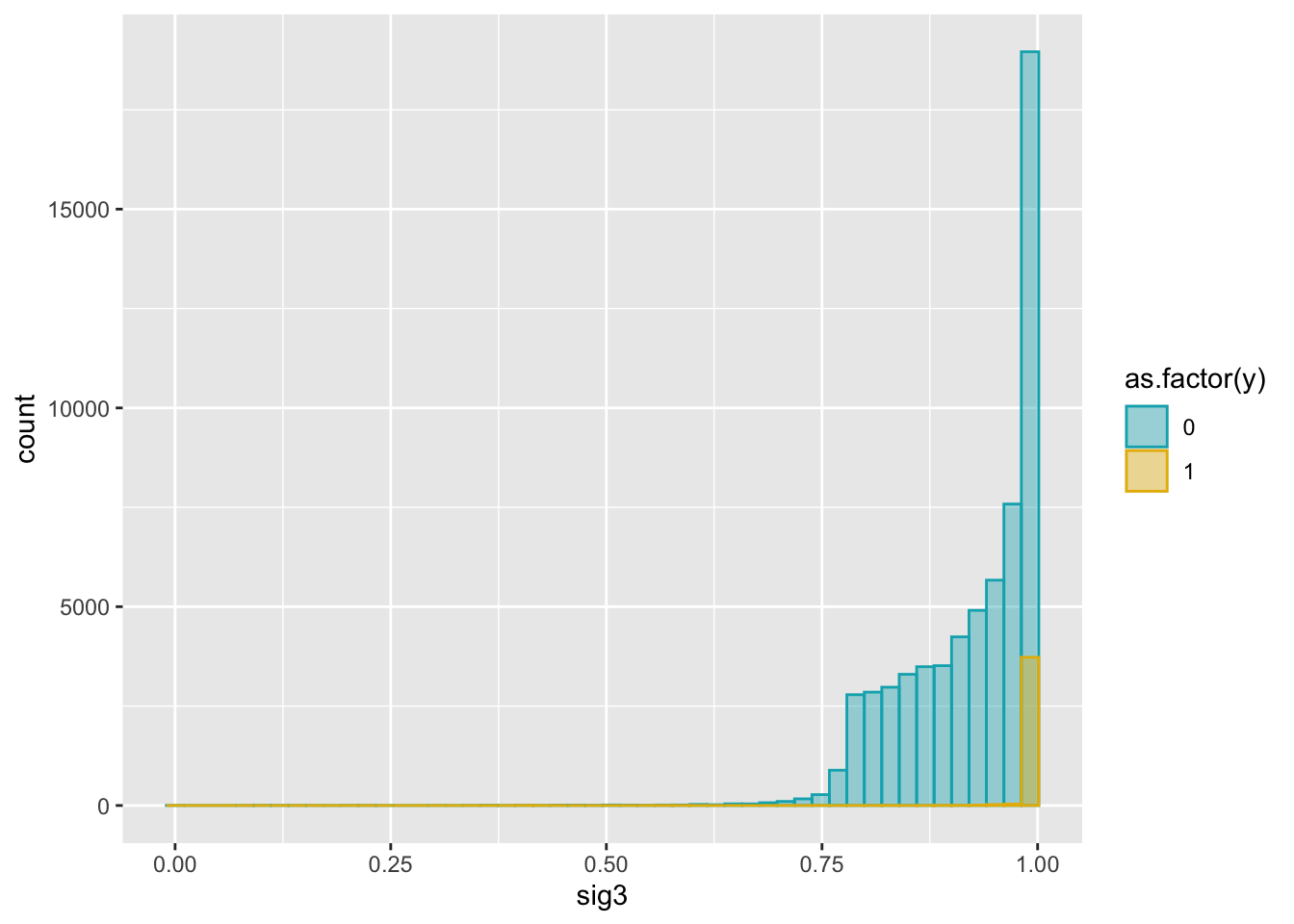

ggplot(dat2, aes(x = sig4)) +
  geom_histogram(aes(color = as.factor(y), fill = as.factor(y)), 
                position = "identity", bins = 50, alpha = 0.4) +
  scale_color_manual(values = c("#00AFBB", "#E7B800")) +
  scale_fill_manual(values = c("#00AFBB", "#E7B800"))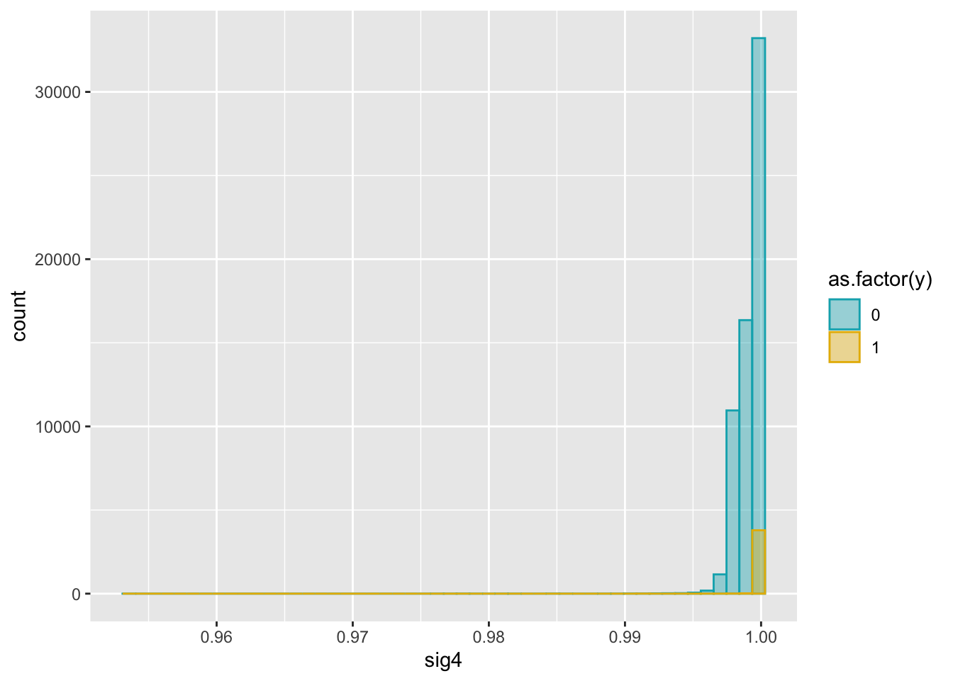

add weight to all feature logsitic regression and plot ROC/PR-AUC

# split data in the same way
set.seed(1)
n = dim(dat2)[1]
indx = sample(1:n, round(2*n/3), replace = FALSE)
train = dat2[indx, ]
test = dat2[-indx, ]

# fit model and evaluate performance
fit.sig1 = glm(y ~ UTR5 + UTR3 + intron + upstream + exon + sig1, data = train, family = "binomial")
fit.sig2 = glm(y ~ UTR5 + UTR3 + intron + upstream + exon + sig2, data = train, family = "binomial")
fit.sig3 = glm(y ~ UTR5 + UTR3 + intron + upstream + exon + sig3, data = train, family = "binomial")

Warning: glm.fit: fitted probabilities numerically 0 or 1 occurred

fit.sig4 = glm(y ~ UTR5 + UTR3 + intron + upstream + exon + sig4, data = train, family = "binomial")

Warning: glm.fit: fitted probabilities numerically 0 or 1 occurred

summary(fit.sig1)


Call:
glm(formula = y ~ UTR5 + UTR3 + intron + upstream + exon + sig1, 
    family = "binomial", data = train)

Deviance Residuals: 
    Min       1Q   Median       3Q      Max  
-2.7492  -0.1679  -0.1679  -0.1679   2.9218  

Coefficients:
            Estimate Std. Error z value Pr(>|z|)    
(Intercept) -4.25439    0.04086 -104.13   <2e-16 ***
UTR5         3.00116    0.24081   12.46   <2e-16 ***
UTR3         2.73910    0.25257   10.85   <2e-16 ***
intron       3.98281    0.09417   42.30   <2e-16 ***
upstream     3.47761    0.22246   15.63   <2e-16 ***
exon         4.04047    0.28095   14.38   <2e-16 ***
sig1         4.01070    0.08689   46.16   <2e-16 ***
---
Signif. codes:  0 '***' 0.001 '**' 0.01 '*' 0.05 '.' 0.1 ' ' 1

(Dispersion parameter for binomial family taken to be 1)

    Null deviance: 19491.1  on 43904  degrees of freedom
Residual deviance:  8537.3  on 43898  degrees of freedom
AIC: 8551.3

Number of Fisher Scoring iterations: 7

summary(fit.sig2)


Call:
glm(formula = y ~ UTR5 + UTR3 + intron + upstream + exon + sig2, 
    family = "binomial", data = train)

Deviance Residuals: 
    Min       1Q   Median       3Q      Max  
-2.2622  -0.0999  -0.0551  -0.0549   3.6049  

Coefficients:
            Estimate Std. Error z value Pr(>|z|)    
(Intercept) -6.49602    0.11369 -57.137   <2e-16 ***
UTR5         4.02543    0.21912  18.371   <2e-16 ***
UTR3         1.96577    0.20603   9.541   <2e-16 ***
intron       3.22338    0.08764  36.782   <2e-16 ***
upstream     3.97905    0.18547  21.454   <2e-16 ***
exon         3.83058    0.25999  14.734   <2e-16 ***
sig2         4.94887    0.13213  37.454   <2e-16 ***
---
Signif. codes:  0 '***' 0.001 '**' 0.01 '*' 0.05 '.' 0.1 ' ' 1

(Dispersion parameter for binomial family taken to be 1)

    Null deviance: 19491.1  on 43904  degrees of freedom
Residual deviance:  7689.3  on 43898  degrees of freedom
AIC: 7703.3

Number of Fisher Scoring iterations: 8

summary(fit.sig3)


Call:
glm(formula = y ~ UTR5 + UTR3 + intron + upstream + exon + sig3, 
    family = "binomial", data = train)

Deviance Residuals: 
    Min       1Q   Median       3Q      Max  
-2.2442  -0.2664  -0.0604  -0.0044   8.4904  

Coefficients:
             Estimate Std. Error z value Pr(>|z|)    
(Intercept) -64.18069    2.95168  -21.74   <2e-16 ***
UTR5          4.88439    0.21454   22.77   <2e-16 ***
UTR3          2.68043    0.20093   13.34   <2e-16 ***
intron        3.79105    0.08351   45.40   <2e-16 ***
upstream      4.76853    0.18044   26.43   <2e-16 ***
exon          4.48146    0.24267   18.47   <2e-16 ***
sig3         61.73039    2.97492   20.75   <2e-16 ***
---
Signif. codes:  0 '***' 0.001 '**' 0.01 '*' 0.05 '.' 0.1 ' ' 1

(Dispersion parameter for binomial family taken to be 1)

    Null deviance: 19491.1  on 43904  degrees of freedom
Residual deviance:  8714.6  on 43898  degrees of freedom
AIC: 8728.6

Number of Fisher Scoring iterations: 11

summary(fit.sig4)


Call:
glm(formula = y ~ UTR5 + UTR3 + intron + upstream + exon + sig4, 
    family = "binomial", data = train)

Deviance Residuals: 
    Min       1Q   Median       3Q      Max  
-2.2425  -0.2722  -0.0703  -0.0054   8.4904  

Coefficients:
              Estimate Std. Error z value Pr(>|z|)    
(Intercept) -5423.3296   265.1349  -20.45   <2e-16 ***
UTR5            4.9368     0.2142   23.05   <2e-16 ***
UTR3            2.7305     0.2008   13.60   <2e-16 ***
intron          3.8373     0.0834   46.01   <2e-16 ***
upstream        4.8205     0.1802   26.74   <2e-16 ***
exon            4.5254     0.2416   18.73   <2e-16 ***
sig4         5420.8228   265.1582   20.44   <2e-16 ***
---
Signif. codes:  0 '***' 0.001 '**' 0.01 '*' 0.05 '.' 0.1 ' ' 1

(Dispersion parameter for binomial family taken to be 1)

    Null deviance: 19491  on 43904  degrees of freedom
Residual deviance:  8804  on 43898  degrees of freedom
AIC: 8818

Number of Fisher Scoring iterations: 11

## sigma1
pred.probs=predict(fit.sig1,test,type="response")
glm.pred = rep(0, length(pred.probs))
glm.pred[pred.probs>0.5]= 1
table(glm.pred, test$y)

        
glm.pred     0     1
       0 20591   575
       1    89   698

fg <- pred.probs[test$y == 1]
bg <- pred.probs[test$y== 0]

# ROC Curve    
roc <- roc.curve(scores.class0 = fg, scores.class1 = bg, curve = T)
plot(roc)

# PR Curve
pr <- pr.curve(scores.class0 = fg, scores.class1 = bg, curve = T)
plot(pr)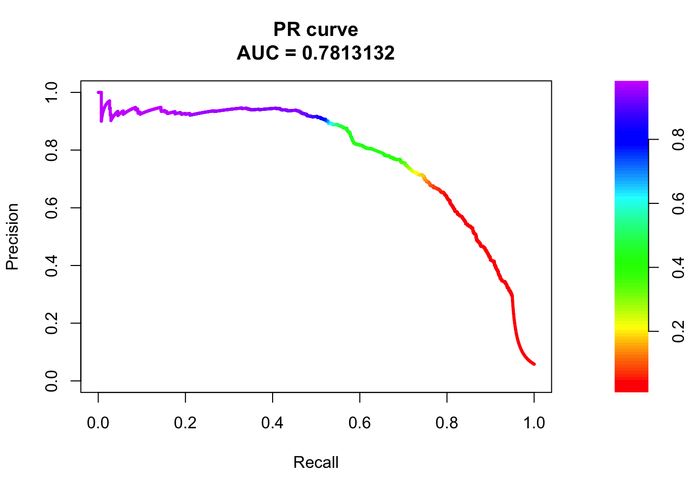

## sigma2
pred.probs=predict(fit.sig2,test,type="response")
glm.pred = rep(0, length(pred.probs))
glm.pred[pred.probs>0.5]= 1
table(glm.pred, test$y)

        
glm.pred     0     1
       0 20528   485
       1   152   788

fg <- pred.probs[test$y == 1]
bg <- pred.probs[test$y== 0]

# ROC Curve    
roc <- roc.curve(scores.class0 = fg, scores.class1 = bg, curve = T)
plot(roc)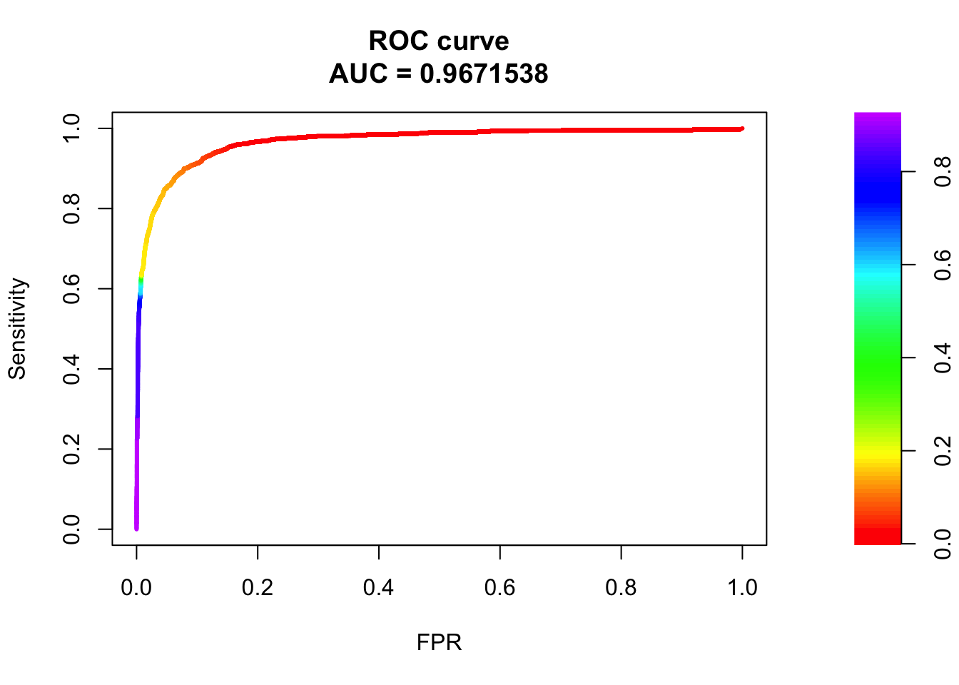

# PR Curve
pr <- pr.curve(scores.class0 = fg, scores.class1 = bg, curve = T)
plot(pr)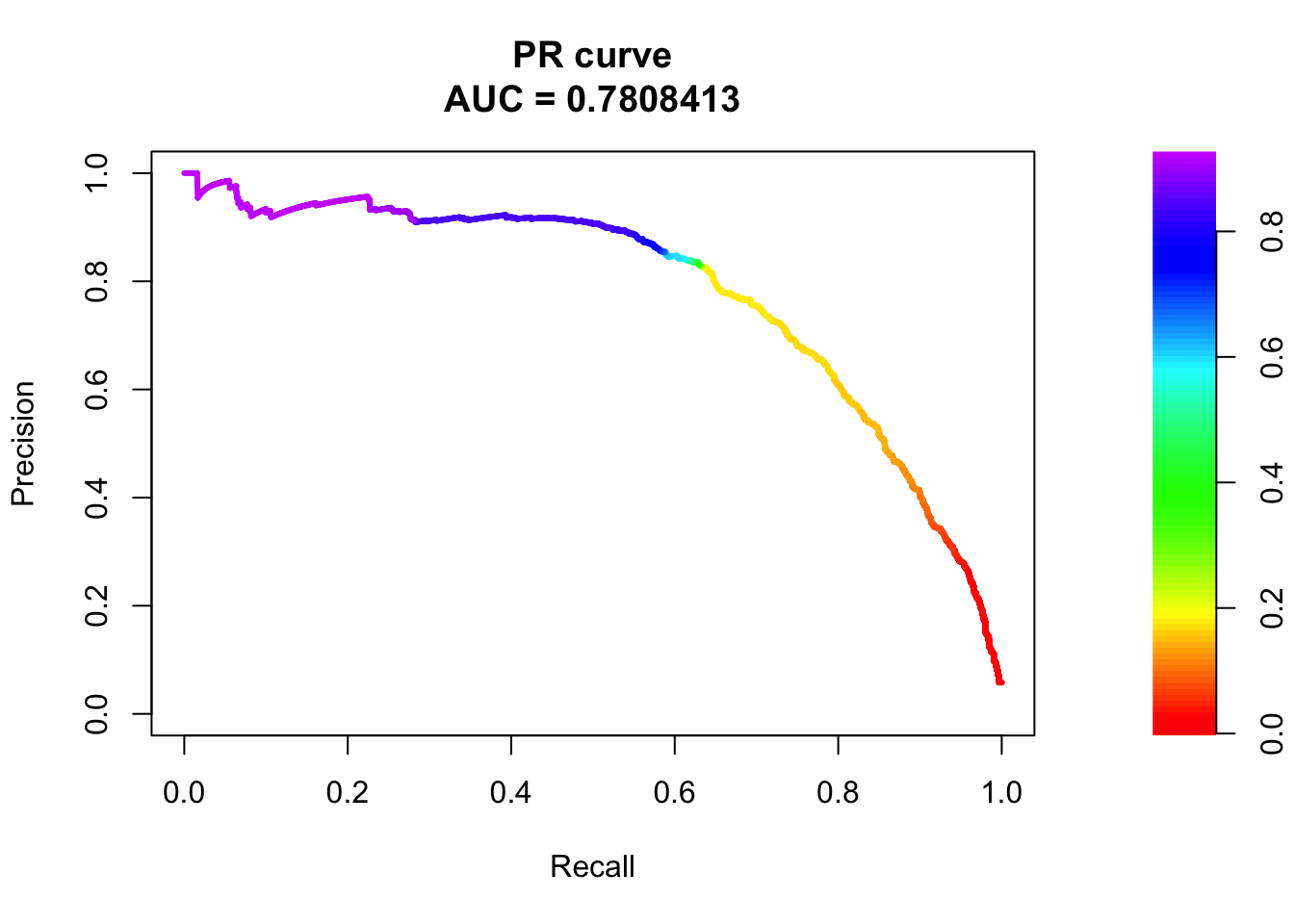

## sigma3
pred.probs=predict(fit.sig3,test,type="response")
glm.pred = rep(0, length(pred.probs))
glm.pred[pred.probs>0.5]= 1
table(glm.pred, test$y)

        
glm.pred     0     1
       0 20505   456
       1   175   817

fg <- pred.probs[test$y == 1]
bg <- pred.probs[test$y== 0]

# ROC Curve    
roc <- roc.curve(scores.class0 = fg, scores.class1 = bg, curve = T)
plot(roc)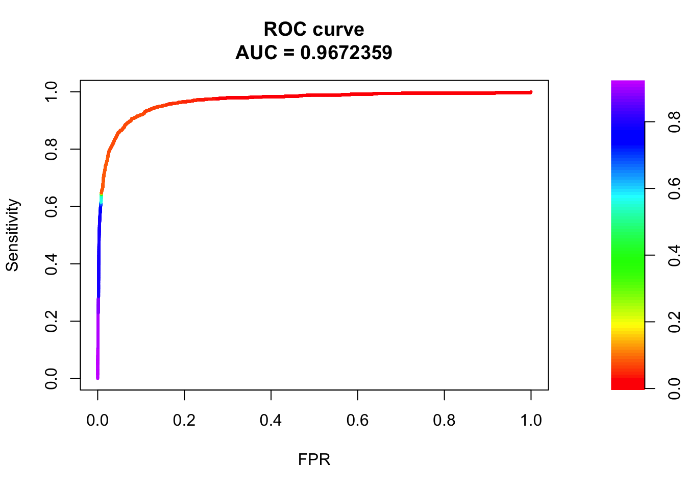

# PR Curve
pr <- pr.curve(scores.class0 = fg, scores.class1 = bg, curve = T)
plot(pr)

## sigma4
pred.probs=predict(fit.sig3,test,type="response")
glm.pred = rep(0, length(pred.probs))
glm.pred[pred.probs>0.5]= 1
table(glm.pred, test$y)

        
glm.pred     0     1
       0 20505   456
       1   175   817

fg <- pred.probs[test$y == 1]
bg <- pred.probs[test$y== 0]

# ROC Curve    
roc <- roc.curve(scores.class0 = fg, scores.class1 = bg, curve = T)
plot(roc)

# PR Curve
pr <- pr.curve(scores.class0 = fg, scores.class1 = bg, curve = T)
plot(pr)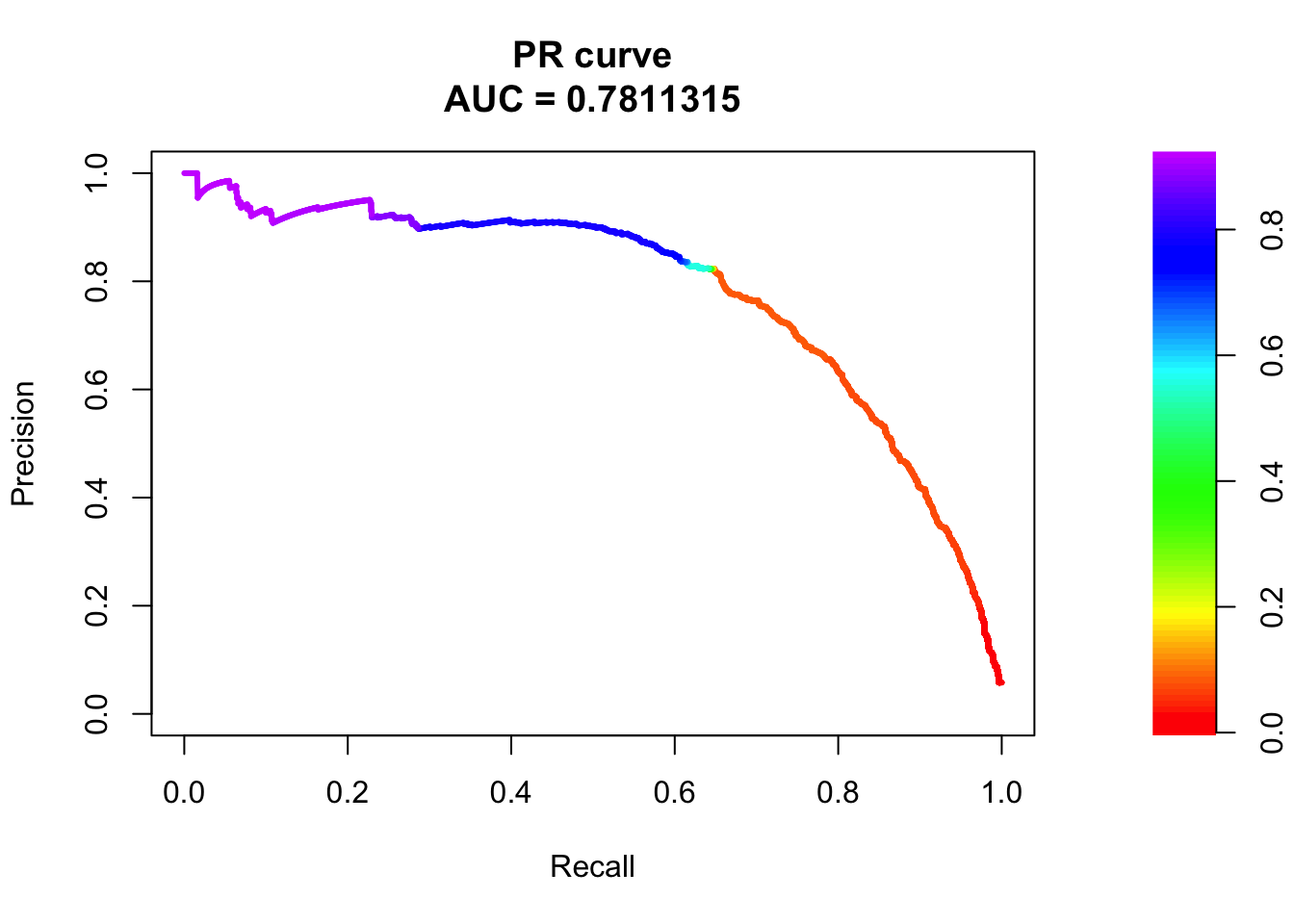

sessionInfo()

R version 3.6.3 (2020-02-29)
Platform: x86_64-apple-darwin15.6.0 (64-bit)
Running under: macOS Catalina 10.15.5

Matrix products: default
BLAS:   /Library/Frameworks/R.framework/Versions/3.6/Resources/lib/libRblas.0.dylib
LAPACK: /Library/Frameworks/R.framework/Versions/3.6/Resources/lib/libRlapack.dylib

locale:
[1] en_US.UTF-8/en_US.UTF-8/en_US.UTF-8/C/en_US.UTF-8/en_US.UTF-8

attached base packages:
[1] stats     graphics  grDevices utils     datasets  methods   base     

other attached packages:
[1] PRROC_1.3.1     dplyr_0.8.5     ggplot2_3.3.0   workflowr_1.6.1

loaded via a namespace (and not attached):
 [1] Rcpp_1.0.4       compiler_3.6.3   pillar_1.4.3     later_1.0.0     
 [5] git2r_0.26.1     highr_0.8        tools_3.6.3      digest_0.6.25   
 [9] evaluate_0.14    lifecycle_0.2.0  tibble_3.0.1     gtable_0.3.0    
[13] pkgconfig_2.0.3  rlang_0.4.5      rstudioapi_0.11  yaml_2.2.1      
[17] xfun_0.12        withr_2.1.2      stringr_1.4.0    knitr_1.28      
[21] fs_1.3.2         vctrs_0.2.4      rprojroot_1.3-2  grid_3.6.3      
[25] tidyselect_1.0.0 glue_1.3.2       R6_2.4.1         rmarkdown_2.1   
[29] farver_2.0.3     purrr_0.3.3      magrittr_1.5     whisker_0.4     
[33] backports_1.1.5  scales_1.1.0     promises_1.1.0   htmltools_0.4.0 
[37] ellipsis_0.3.0   assertthat_0.2.1 colorspace_1.4-1 httpuv_1.5.2    
[41] labeling_0.3     stringi_1.4.6    munsell_0.5.0    crayon_1.3.4

distance function

Yunqi Yang

7/29/2020

Comment:

data overview

proportion of features

play around tss feature

two decay functions: exponential decay and gaussian decay.

exponential decay: exp(-d/sigma)

add weight to all feature logsitic regression and plot ROC/PR-AUC

change to gaussian decay function: \(exp(-d^2/2l^2)\)

add weight to all feature logsitic regression and plot ROC/PR-AUC