distal_feature

workflowr

• Summary
• Checks
• Past versions

Last updated: 2020-09-16

Checks: 6 1

Knit directory: gene_level_fine_mapping/

This reproducible R Markdown analysis was created with workflowr (version 1.6.1). The Checks tab describes the reproducibility checks that were applied when the results were created. The Past versions tab lists the development history.

---

R Markdown file: up-to-date

Great! Since the R Markdown file has been committed to the Git repository, you know the exact version of the code that produced these results.

Environment: empty

Great job! The global environment was empty. Objects defined in the global environment can affect the analysis in your R Markdown file in unknown ways. For reproduciblity it’s best to always run the code in an empty environment.

Seed: set.seed(20200622)

The command set.seed(20200622) was run prior to running the code in the R Markdown file. Setting a seed ensures that any results that rely on randomness, e.g. subsampling or permutations, are reproducible.

Session information: recorded

Great job! Recording the operating system, R version, and package versions is critical for reproducibility.

Cache: none

Nice! There were no cached chunks for this analysis, so you can be confident that you successfully produced the results during this run.

File paths: absolute

Using absolute paths to the files within your workflowr project makes it difficult for you and others to run your code on a different machine. Change the absolute path(s) below to the suggested relative path(s) to make your code more reproducible.

absolute	relative
/Users/nicholeyang/Desktop/gene_level_fine_mapping/data/train_all.RData	data/train_all.RData

Repository version: 6bae65f

Great! You are using Git for version control. Tracking code development and connecting the code version to the results is critical for reproducibility.

The results in this page were generated with repository version 6bae65f. See the Past versions tab to see a history of the changes made to the R Markdown and HTML files.

Note that you need to be careful to ensure that all relevant files for the analysis have been committed to Git prior to generating the results (you can use wflow_publish or wflow_git_commit). workflowr only checks the R Markdown file, but you know if there are other scripts or data files that it depends on. Below is the status of the Git repository when the results were generated:

Ignored files:
    Ignored:    .DS_Store
    Ignored:    .Rhistory
    Ignored:    .Rproj.user/
    Ignored:    analysis/.DS_Store
    Ignored:    analysis/.RData
    Ignored:    analysis/.Rhistory

Untracked files:
    Untracked:  analysis/atac_eqtl.Rmd
    Untracked:  data/hic_eqtl.RData
    Untracked:  data/train_add_hic.RData
    Untracked:  data/train_all.RData

Unstaged changes:
    Modified:   analysis/add_hic_feature.Rmd

Note that any generated files, e.g. HTML, png, CSS, etc., are not included in this status report because it is ok for generated content to have uncommitted changes.

---

These are the previous versions of the repository in which changes were made to the R Markdown (analysis/assess_distal_observation.Rmd) and HTML (docs/assess_distal_observation.html) files. If you’ve configured a remote Git repository (see ?wflow_git_remote), click on the hyperlinks in the table below to view the files as they were in that past version.

File	Version	Author	Date	Message
Rmd	6bae65f	yunqiyang0215	2020-09-16	wflow_publish(“analysis/assess_distal_observation.Rmd”)
html	d6daf14	yunqiyang0215	2020-09-16	Build site.
Rmd	d7d76a2	yunqiyang0215	2020-09-16	wflow_publish(“analysis/assess_distal_observation.Rmd”)
html	fd1c97c	yunqiyang0215	2020-09-16	Build site.
Rmd	8858090	yunqiyang0215	2020-09-16	wflow_publish(“analysis/assess_distal_observation.Rmd”)
html	19966f6	yunqiyang0215	2020-09-16	Build site.
Rmd	a6a1c0f	yunqiyang0215	2020-09-16	wflow_publish(“analysis/assess_distal_observation.Rmd”)
html	20ce646	yunqiyang0215	2020-09-16	Build site.
Rmd	b1e3ea3	yunqiyang0215	2020-09-16	wflow_publish(“analysis/assess_distal_observation.Rmd”)
html	1d0f053	yunqiyang0215	2020-08-31	Build site.
html	a187678	yunqiyang0215	2020-08-31	Build site.
Rmd	a494940	yunqiyang0215	2020-08-31	wflow_publish(“analysis/assess_distal_observation.Rmd”)
html	bcf3283	yunqiyang0215	2020-08-31	Build site.
Rmd	50aca89	yunqiyang0215	2020-08-31	wflow_publish(“analysis/assess_distal_observation.Rmd”)

---

Description:

1. model the distal observations, tss_dist_to_snp > 100kb

2. the feature weight, HIC and ATAC have no prediction power, predict all the observations to be negative.

3. If adding all other functional features, including exon, intron,…, that improve the classification performance. The accuracy is still not high, \(9/49\approx0.184\).

4. The important questions here:

(1). why we couldn’t classify distal observations well?

(2). why intron/exon(features in closer range) better than distal features?

The problem of the eQTL data? The problem of the HiC ATAC feature data?

Possible next step:

1. Instead of using binary outcome y, do more exploratory analysis on PIP, to see if there’s relationship between PIP and distance.

2. Relax eQTL PIP threshold to include more into training data. To see if distal pairs increase or not. If not, this means that eQTL couldn’t capture distal gene-snp association or the calculation of PIP doesn’t consider distal interaction.

library(ggplot2)
library(dplyr)

Attaching package: 'dplyr'

The following objects are masked from 'package:stats':

    filter, lag

The following objects are masked from 'package:base':

    intersect, setdiff, setequal, union

require(PRROC)

Loading required package: PRROC

load('/Users/nicholeyang/Desktop/gene_level_fine_mapping/data/train_all.RData')
head(train_all_sig)

  gene_name      snp_loc38             variant_id UTR5 UTR3 exon intron
1      A1BG chr19:57866502 chr19_57866502_T_C_b38    0    0    0      0
2      A1BG chr19:58059544 chr19_58059544_T_G_b38    0    0    0      0
3      A1BG chr19:58170494 chr19_58170494_G_T_b38    0    0    0      0
4      A1BG chr19:58228973 chr19_58228973_T_G_b38    0    0    0      0
5      A1BG chr19:58330182 chr19_58330182_C_T_b38    0    0    0      0
6      A1BG chr19:58359927 chr19_58359927_G_A_b38    0    0    0      0
  upstream tss_dist_to_snp y Mon Mac0 Mac1 Mac2 Neu MK EP Ery FoeT nCD4 tCD4
1        0          481132 0   0    0    0    0   0  0  0   0    0    0    0
2        0          288090 0   0    0    0    0   0  0  0   0    0    0    0
3        0          177140 0   0    0    0    0   0  0  0   0    0    0    0
4        0          118661 0   0    0    0    0   0  0  0   0    0    0    0
5        0           17452 1   0    0    0    0   0  0  0   0    0    0    0
6        0            6428 1   0    0    0    0   0  0  0   0    0    0    0
  aCD4 naCD4 nCD8 tCD8 nB tB correlation
1    0     0    0    0  0  0           0
2    0     0    0    0  0  0           0
3    0     0    0    0  0  0           0
4    0     0    0    0  0  0           0
5    0     0    0    0  0  0           0
6    0     0    0    0  0  0           0

process all features

# create unified HiC feature
hic = apply(train_all_sig[, c(11:27)], 1, sum)
train_all_sig$hic = ifelse(hic>0, 1, 0)

# ATAC data
train_all_sig$atac = ifelse(train_all_sig$correlation > 0.5, 1, 0)

# transform tss_dist_to_snp into weights 
sigma = 1e5
train_all_sig$weight = exp(-train_all_sig$tss_dist_to_snp/sigma)

dat = train_all_sig[train_all_sig$tss_dist_to_snp > 1e5, ]

sum(dat$y == 1)

[1] 146

sum(dat$y == 0)

[1] 48505

Create a training/test set

set.seed(215)

n = dim(dat)[1]
indx = sample(1:n, round(2*n/3), replace = FALSE)
train = dat[indx, ]
test = dat[-indx, ]

sum(train$y == 1)

[1] 97

fit1: model contains weight + most of the features

fit1 = glm(y ~ weight + exon + UTR5 + UTR3+ intron+ upstream, data = train, family = "binomial")
summary(fit1)

Call:
glm(formula = y ~ weight + exon + UTR5 + UTR3 + intron + upstream, 
    family = "binomial", data = train)

Deviance Residuals: 
    Min       1Q   Median       3Q      Max  
-1.8093  -0.0680  -0.0545  -0.0500   3.6803  

Coefficients:
            Estimate Std. Error z value Pr(>|z|)    
(Intercept)  -6.7714     0.1884 -35.938  < 2e-16 ***
weight        4.9461     0.9517   5.197 2.02e-07 ***
exon          7.2503     1.1756   6.167 6.95e-10 ***
UTR5          5.4269     1.2719   4.267 1.98e-05 ***
UTR3          5.6461     0.8176   6.906 4.98e-12 ***
intron        5.8104     0.3403  17.072  < 2e-16 ***
upstream      5.5072     1.2500   4.406 1.05e-05 ***
---
Signif. codes:  0 '***' 0.001 '**' 0.01 '*' 0.05 '.' 0.1 ' ' 1

(Dispersion parameter for binomial family taken to be 1)

    Null deviance: 1321.3  on 32433  degrees of freedom
Residual deviance: 1019.5  on 32427  degrees of freedom
AIC: 1033.5

Number of Fisher Scoring iterations: 9

pred.probs=predict(fit1,test,type="response")
glm.pred = rep(0, length(pred.probs))


## all predicted to be negative
glm.pred[pred.probs>0.5]= 1
table(glm.pred, test$y)

        
glm.pred     0     1
       0 16162    40
       1     6     9

# prediction accuracy
accuracy = sum(glm.pred == test$y)/length(test$y)
accuracy 

[1] 0.9971635

fg <- pred.probs[test$y == 1]
bg <- pred.probs[test$y== 0]

# ROC Curve    
roc <- roc.curve(scores.class0 = fg, scores.class1 = bg, curve = T)
plot(roc)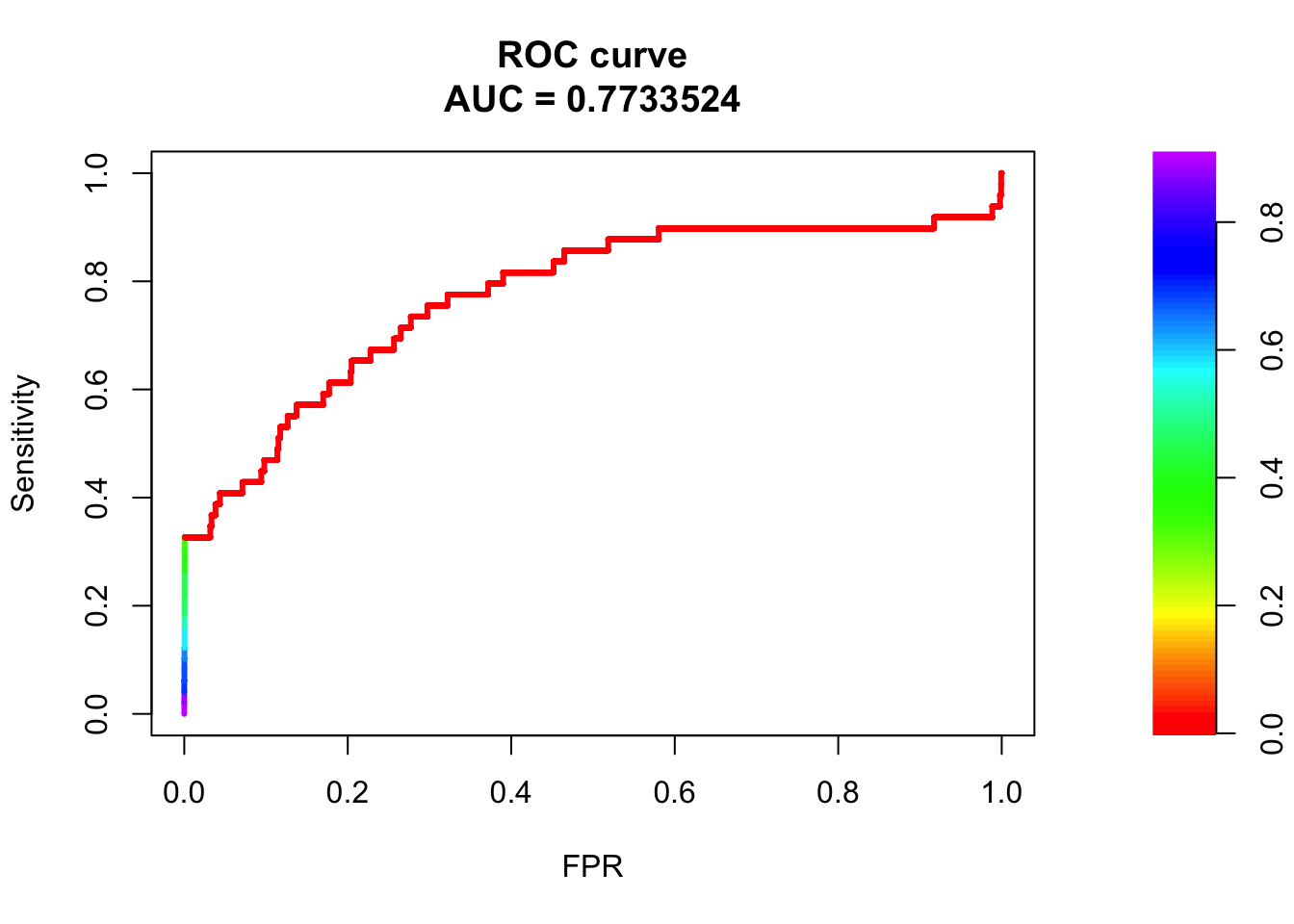

Past versions of unnamed-chunk-8-1.png

Version	Author	Date
20ce646	yunqiyang0215	2020-09-16
bcf3283	yunqiyang0215	2020-08-31

# PR Curve
pr <- pr.curve(scores.class0 = fg, scores.class1 = bg, curve = T)
plot(pr)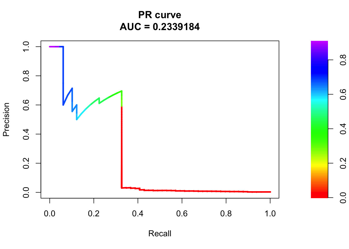

Past versions of unnamed-chunk-8-2.png

Version	Author	Date
20ce646	yunqiyang0215	2020-09-16
bcf3283	yunqiyang0215	2020-08-31

fit2: model contains weight + exon

fit2 = glm(y ~ weight + exon, data = train, family = "binomial")
summary(fit2)

Call:
glm(formula = y ~ weight + exon, family = "binomial", data = train)

Deviance Residuals: 
    Min       1Q   Median       3Q      Max  
-1.8546  -0.0794  -0.0596  -0.0534   3.6508  

Coefficients:
            Estimate Std. Error z value Pr(>|z|)    
(Intercept)  -6.6632     0.1801 -36.994  < 2e-16 ***
weight        6.3711     0.8650   7.365 1.77e-13 ***
exon          6.9730     1.1844   5.887 3.93e-09 ***
---
Signif. codes:  0 '***' 0.001 '**' 0.01 '*' 0.05 '.' 0.1 ' ' 1

(Dispersion parameter for binomial family taken to be 1)

    Null deviance: 1321.3  on 32433  degrees of freedom
Residual deviance: 1240.8  on 32431  degrees of freedom
AIC: 1246.8

Number of Fisher Scoring iterations: 9

pred.probs=predict(fit2,test,type="response")
glm.pred = rep(0, length(pred.probs))


## all predicted to be negative
glm.pred[pred.probs>0.5]= 1
table(glm.pred, test$y)

        
glm.pred     0     1
       0 16167    46
       1     1     3

# prediction accuracy
accuracy = sum(glm.pred == test$y)/length(test$y)
accuracy 

[1] 0.9971018

fg <- pred.probs[test$y == 1]
bg <- pred.probs[test$y== 0]

# ROC Curve    
roc <- roc.curve(scores.class0 = fg, scores.class1 = bg, curve = T)
plot(roc)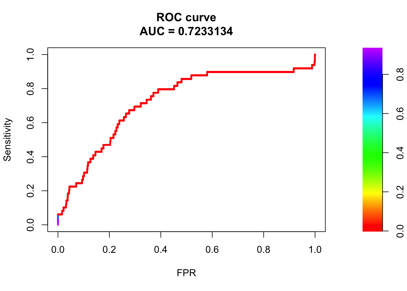

Past versions of unnamed-chunk-11-1.png

Version	Author	Date
20ce646	yunqiyang0215	2020-09-16
bcf3283	yunqiyang0215	2020-08-31

# PR Curve
pr <- pr.curve(scores.class0 = fg, scores.class1 = bg, curve = T)
plot(pr)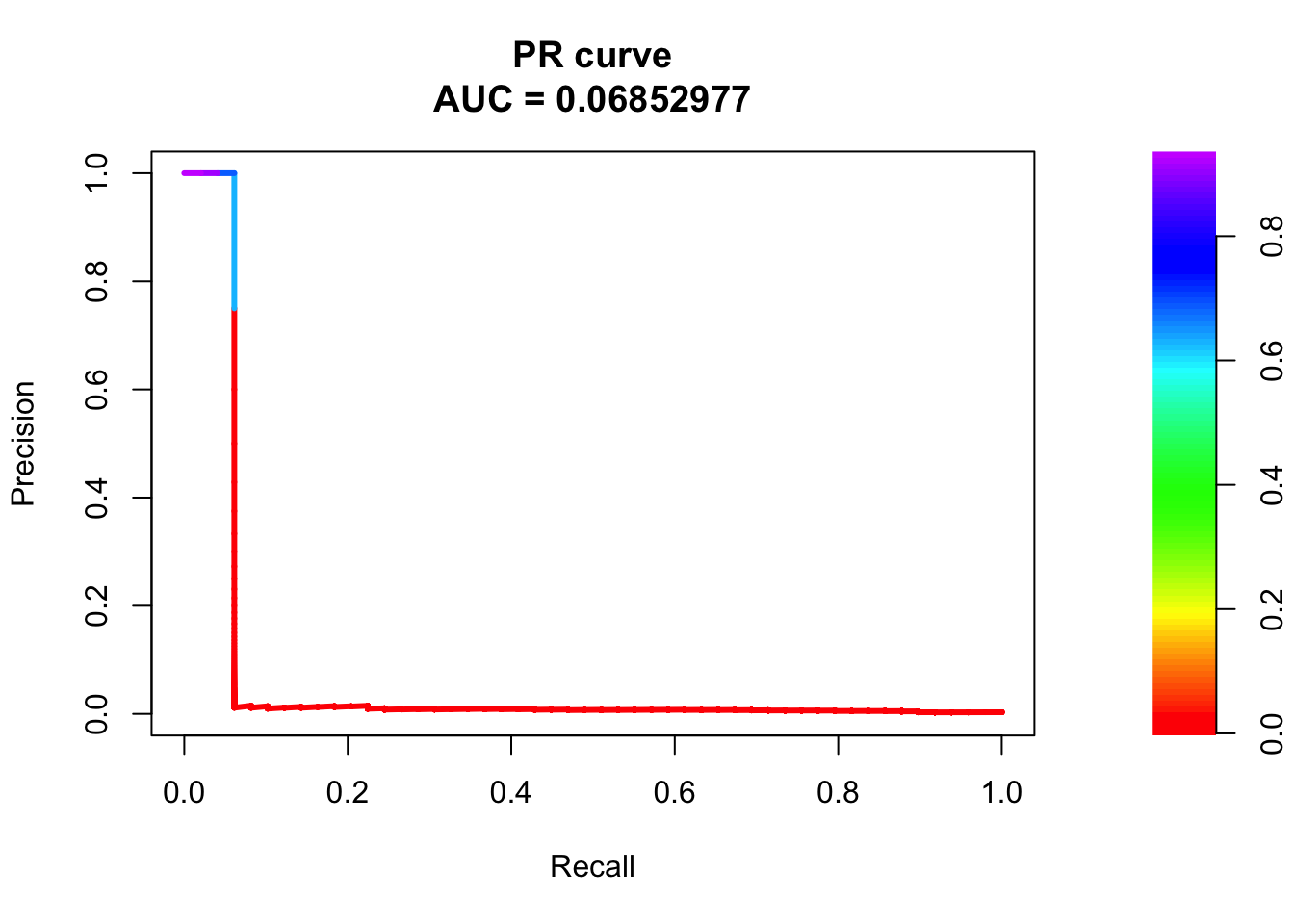

Past versions of unnamed-chunk-11-2.png

Version	Author	Date
20ce646	yunqiyang0215	2020-09-16
bcf3283	yunqiyang0215	2020-08-31

fit3: model only contains weight

fit3 = glm(y ~ weight, data = train, family = "binomial")
summary(fit3)

Call:
glm(formula = y ~ weight, family = "binomial", data = train)

Deviance Residuals: 
    Min       1Q   Median       3Q      Max  
-0.1640  -0.0808  -0.0608  -0.0546   3.6389  

Coefficients:
            Estimate Std. Error z value Pr(>|z|)    
(Intercept)  -6.6200     0.1768 -37.433  < 2e-16 ***
weight        6.3019     0.8532   7.386 1.51e-13 ***
---
Signif. codes:  0 '***' 0.001 '**' 0.01 '*' 0.05 '.' 0.1 ' ' 1

(Dispersion parameter for binomial family taken to be 1)

    Null deviance: 1321.3  on 32433  degrees of freedom
Residual deviance: 1271.1  on 32432  degrees of freedom
AIC: 1275.1

Number of Fisher Scoring iterations: 9

pred.probs=predict(fit3,test,type="response")
glm.pred = rep(0, length(pred.probs))


## all predicted to be negative
glm.pred[pred.probs>0.5]= 1
table(glm.pred, test$y)

        
glm.pred     0     1
       0 16168    49

# prediction accuracy
accuracy = sum(glm.pred == test$y)/length(test$y)
accuracy 

[1] 0.9969785

fg <- pred.probs[test$y == 1]
bg <- pred.probs[test$y== 0]

# ROC Curve    
roc <- roc.curve(scores.class0 = fg, scores.class1 = bg, curve = T)
plot(roc)

Past versions of unnamed-chunk-14-1.png

Version	Author	Date
20ce646	yunqiyang0215	2020-09-16

# PR Curve
pr <- pr.curve(scores.class0 = fg, scores.class1 = bg, curve = T)
plot(pr)

Past versions of unnamed-chunk-14-2.png

Version	Author	Date
20ce646	yunqiyang0215	2020-09-16

fit4: model contains weight, HiC and ATAC

fit4 = glm(y ~ weight + hic + atac, data = train, family = "binomial")
summary(fit4)

Call:
glm(formula = y ~ weight + hic + atac, family = "binomial", data = train)

Deviance Residuals: 
    Min       1Q   Median       3Q      Max  
-0.2994  -0.0809  -0.0591  -0.0527   3.6589  

Coefficients:
            Estimate Std. Error z value Pr(>|z|)    
(Intercept) -6.69306    0.18309 -36.557  < 2e-16 ***
weight       6.32761    0.86039   7.354 1.92e-13 ***
hic         -0.01067    0.27603  -0.039  0.96915    
atac         1.31793    0.35309   3.733  0.00019 ***
---
Signif. codes:  0 '***' 0.001 '**' 0.01 '*' 0.05 '.' 0.1 ' ' 1

(Dispersion parameter for binomial family taken to be 1)

    Null deviance: 1321.3  on 32433  degrees of freedom
Residual deviance: 1261.1  on 32430  degrees of freedom
AIC: 1269.1

Number of Fisher Scoring iterations: 9

pred.probs=predict(fit4,test,type="response")
glm.pred = rep(0, length(pred.probs))

## all predicted to be negative 
glm.pred[pred.probs>0.5]= 1
table(glm.pred, test$y)

        
glm.pred     0     1
       0 16168    49

# prediction accuracy
accuracy = sum(glm.pred == test$y)/length(test$y)
accuracy 

[1] 0.9969785

fg <- pred.probs[test$y == 1]
bg <- pred.probs[test$y== 0]

# ROC Curve    
roc <- roc.curve(scores.class0 = fg, scores.class1 = bg, curve = T)
plot(roc)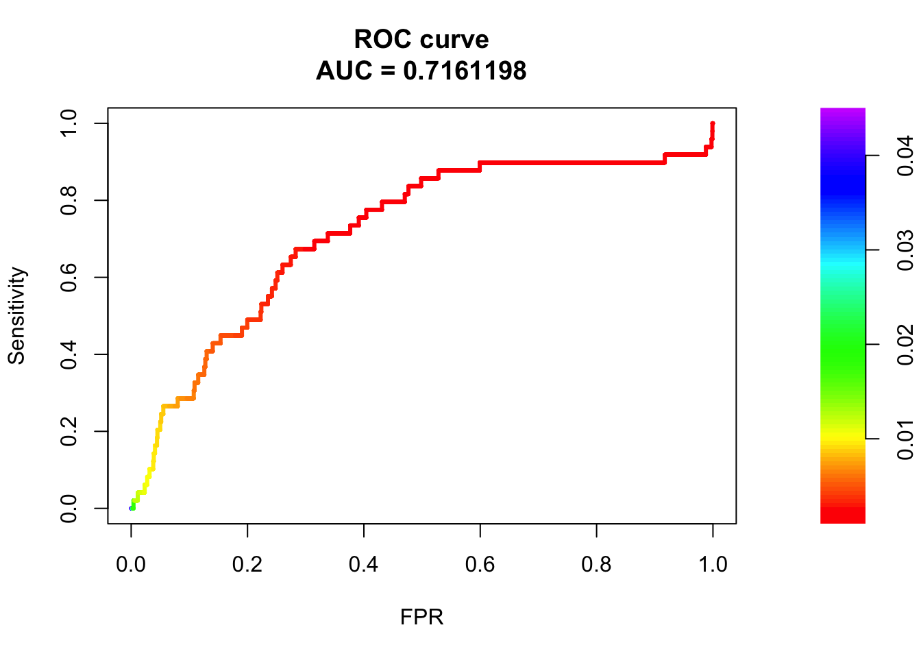

Past versions of unnamed-chunk-17-1.png

Version	Author	Date
20ce646	yunqiyang0215	2020-09-16

# PR Curve
pr <- pr.curve(scores.class0 = fg, scores.class1 = bg, curve = T)
plot(pr)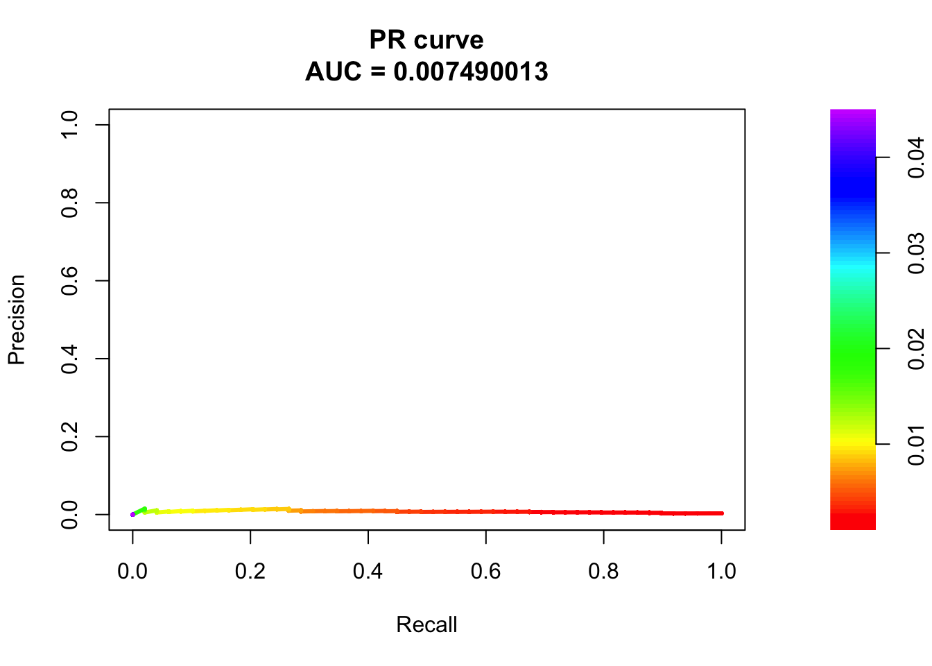

Past versions of unnamed-chunk-17-2.png

Version	Author	Date
20ce646	yunqiyang0215	2020-09-16

More exploratory analysis:

## proportion of positive observations by distance
sum(dat$y == 1)/dim(dat)[1]   ## distal ones 

[1] 0.003000966

sum(train_all_sig$y == 1)/dim(train_all_sig)[1]

[1] 0.05779677

Session information

sessionInfo()

R version 3.6.3 (2020-02-29)
Platform: x86_64-apple-darwin15.6.0 (64-bit)
Running under: macOS Catalina 10.15.5

Matrix products: default
BLAS:   /Library/Frameworks/R.framework/Versions/3.6/Resources/lib/libRblas.0.dylib
LAPACK: /Library/Frameworks/R.framework/Versions/3.6/Resources/lib/libRlapack.dylib

locale:
[1] en_US.UTF-8/en_US.UTF-8/en_US.UTF-8/C/en_US.UTF-8/en_US.UTF-8

attached base packages:
[1] stats     graphics  grDevices utils     datasets  methods   base     

other attached packages:
[1] PRROC_1.3.1     dplyr_0.8.5     ggplot2_3.3.0   workflowr_1.6.1

loaded via a namespace (and not attached):
 [1] Rcpp_1.0.4       compiler_3.6.3   pillar_1.4.3     later_1.0.0     
 [5] git2r_0.26.1     highr_0.8        tools_3.6.3      digest_0.6.25   
 [9] evaluate_0.14    lifecycle_0.2.0  tibble_3.0.1     gtable_0.3.0    
[13] pkgconfig_2.0.3  rlang_0.4.5      rstudioapi_0.11  yaml_2.2.1      
[17] xfun_0.12        withr_2.1.2      stringr_1.4.0    knitr_1.28      
[21] fs_1.3.2         vctrs_0.2.4      rprojroot_1.3-2  grid_3.6.3      
[25] tidyselect_1.0.0 glue_1.3.2       R6_2.4.1         rmarkdown_2.1   
[29] purrr_0.3.3      magrittr_1.5     whisker_0.4      backports_1.1.5 
[33] scales_1.1.0     promises_1.1.0   htmltools_0.4.0  ellipsis_0.3.0  
[37] assertthat_0.2.1 colorspace_1.4-1 httpuv_1.5.2     stringi_1.4.6   
[41] munsell_0.5.0    crayon_1.3.4